K-PD models | Mlxtran

Usual PK-PD models describe the relationships between dose regimens, drug concentration and effect (or response). They are applied when both the drug concentration and the effect can be measured. However situations exist where the concentration PK data is not available. This may for instance be the case for phase III clinical trials or pediatric studies. In this case K-PD models can be used: the drug concentration-effect relationship model is kept, but the (unobserved) PK profile is assumed to have a simple shape. In comparison to dose-response studies which directly link the (constant) dose to the PD response, K-PD models permit to capture PD profile that varies over time as a consequence of the underlying time-varying PK profile.

Although not being the first published example of K-PD model, the usual reference is:

Jacqmin, P., Snoeck, E., Schaick, E. A. Van, Gieschke, R., Pillai, P., Steimer, J., & Girard, P. (2007). Modelling Response Time Profiles in the Absence of Drug Concentrations : Definition and Performance Evaluation of the K-PD Model. Journal of Pharmacokinetics and Pharmacodynamics, 34(1).

Mlxtran code for K-PD models

The effect of the drug on the response can be as diverse as presented in the indirect response models and direct response models examples. We here focus on the case of an indirect response where the drug decreases the response production rate.

Formulation by Jacqmin et al.

The authors in Jacqmin et al. describe the model in the following way: “A virtual compartment representing the biophase in which the concentration is in equilibrium with the observed effect is used to extract the (pharmaco)kinetic component from the pharmacodynamic data alone. Parameters of this model are the elimination rate constant from the virtual compartment (KDE), which describes the equilibrium between the rate of dose administration and the observed effect, and the second parameter, named EDK50 which is the apparent in vivo potency of the drug at steady state.

The equations read:

$\frac{dA}{dt} = - \textrm{KDE} \times A$

$\textrm{IR} = \textrm{KDE} \times A$

$\frac{dR}{dt} = K_s \left(1-\frac{\textrm{IR}}{\textrm{EDK}_{50} + \textrm{IR}} \right) - K_D R$

with A the drug amount, R the response, KDE the drug elimination rate, Ks the response synthesis rate, Kd the response disappearance rate constant. EDK50 represents the potency of the drug and also corresponds to EDK50 constant corresponds to the product of the EC50 and the clearance.

The corresponding Mlxtran code is:

[LONGITUDINAL]
input={Ks,Kd,KDE,EDK50}

PK:
depot(target=A)

EQUATION:
; initialization
t_0 = 0
A_0 = 0
R_0 = Ks/Kd

; ODEs
ddt_A = - KDE*A
ddt_R = Ks * (1 - (KDE*A)/(EDK50 + (KDE*A))) - Kd*R

OUTPUT:
output = {R}

Note that the only output is the response R, as only the response has been measured and recorded in the data set.

Alternative formulation

For some applications, the interpretation of the parameters of the Jacqmin model may be difficult. It is also unusual the consider that it is the rate at which the drug disappear (IR) that drives the effect on the response. We thus propose an alternative formulation of the same model.

We start by writing the model using the usual (and physiologically relevant) effect of the drug concentration on the response:

$\frac{dA}{dt} = - \textrm{KDE} \times A$

$C_A = \frac{A}{V_A}$

$\frac{dR}{dt} = K_s \left(1-\frac{C_A}{\textrm{IC}_{50} + C_A} \right) - K_D R$

This set of equations can be rewritten into:

$\frac{dA}{dt} = - \textrm{KDE} \times A$

$\frac{dR}{dt} = K_s \left(1-\frac{A}{\textrm{IC}_{50} \times V_A + A} \right) - K_D R$

using the fact that $C_A=\frac{A}{V_A}$ . When the drug concentration is observed, it is possible to identify both $V_A$ and $\textrm{IC}_{50}$ separately because $V_A$ influences the observed drug concentration. However when the drug concentration is not measured, it is not possible to identify both $V_A$ and $\textrm{IC}_{50}$ , but only the product of the two. The unidentifiability of the volume of distribution is explore visually and interactively in the next section.

We thus introduce $\textrm{A}_{50}=\textrm{IC}_{50} \times V_A$ and write our final model as:

$\frac{dA}{dt} = - \textrm{KDE} \times A$

$\frac{dR}{dt} = K_s \left(1-\frac{A}{\textrm{A}_{50} + A} \right) - K_D R$

The parameter $\textrm{A}_{50}$ can simply be interpreted as the product of the usual $\textrm{IC}_{50}$ and the volume of distribution $V_A$ of the drug.

The mlxtran model reads:

[LONGITUDINAL]
input={Ks,Kd,KDE,A50}

PK:
depot(target=A)

EQUATION:
; initialization
t_0 = 0
A_0 = 0
R_0 = Ks/Kd

; ODEs
ddt_A = - KDE*A
ddt_R = Ks * (1 - A/(A50 + A) ) - Kd*R

OUTPUT:
output = {R}

The model can also be written using macros for the (P)K part. When macros are used, the PK part of the model will be calculated using the analytical solution while the PD part will be solved using the ODE solver.

[LONGITUDINAL] 
input={Ks,Kd,KDE,A50} 

PK: 
compartment(cmt=1, amount=A)
iv(cmt=1)
elimination(cmt=1, k=KDE) 

EQUATION: 
; initialization 
t_0 = 0 
R_0 = Ks/Kd 

; ODEs 
ddt_R = Ks * (1 - A/(A50 + A) ) - Kd*R 

OUTPUT: 
output = {R}

Extensions

If data is sufficient to allow for the estimation of the additional parameters, the model can be extended, for instance in the following directions:

more complex profile for the drug concentration, for example with a first-order input rate. In this case, the additional input arguments can be directly given in the depot macro.
sigmoïdal Emax or Imax model with a hill exponent
Emax or Imax value different from one

The model can also be adapted to consider K-PK models, where two drugs interact and only one of the two is measured.

Simplifications

The use of an Emax or Imax model is only suited if the dose range is sufficiently large to cover both the linear and saturating part of the Michaelis-Menten curve. If concentrations are always smaller than the EC50, the model simplifies to:

$\frac{dA}{dt} = - \textrm{KDE} \times A$

$\frac{dR}{dt} = K_s \left(1- K_e \times A \right) - K_D R$

test

Exploration of the unidentifiability of the drug volume of distribution with Mlxplore

In the section above, we have seen why the volume of distribution is not identifiable from a mathematical point of view. In this section, we explore this unidentifiability interactively with Mlxplore.

The following Mlxplore script defines the model (using the alternative formulation and including the volume), the reference parameter values, an arbitrary dose for A and the simulation output:

<MODEL>
[LONGITUDINAL]
input={Ks,Kd,KDE,IC50,V}

EQUATION:
; initialization
t_0 = 0
A_0 = 0
R_0 = Ks/Kd

; ODEs
ddt_A = - KDE*A
CA = A/V
ddt_R = Ks * (1 - CA/(IC50 + CA) ) - Kd*R

OUTPUT:
output = {R}

<PARAMETER>
KDE=0.5
IC50=50
Ks=0.1
Kd = 0.01
V=1

<DESIGN>
[ADMINISTRATION]
adm={amount=100, time=0, target=A}

<OUTPUT>
list={A,CA,R}
grid=-1:0.1:50

<RESULTS>
[GRAPHICS]
p1 = {y=A, ylabel='Assumed drug amount', xlabel='Time'}
p2 = {y=CA, ylabel='Assumed drug concentration', xlabel='Time'}
p3 = {y=R, ylabel='Indirect response', xlabel='Time'}

Using the sliders to play with the parameter values, it can easily be seen that several sets of parameters lead to the same prediction for the response, compare for instance (V=1,IC50=50) and (V=2,IC50=25). The drug concentration on the opposite is not the same, but as it is not measured, it cannot help in identifying uniquely V and IC50.

In the figure below, we see the drug amount in blue, the drug concentration in orange and the response in green. The first set of parameters is displayed in light colors and the second set in darker colors.

Comparison of dose-response and K-PD approaches for the indirect model with Mlxplore

When an indirect response model is used, it is also common to do a dose-response approach, where the response is directly influenced by the dose instead of the drug concentration as in the K-PD approach. In this section, we will compare the two methods and see when one or the other is more appropriate.

The equation for the dose-response approach is:

$\frac{dR}{dt} = K_s \left(1-\frac{\textrm{DOSE}}{\textrm{D}_{50} + \textrm{DOSE}} \right) - K_D R$

As a reminder, the equations for the K-PD model are:

$\frac{dA}{dt} = - \textrm{KDE} \times A$

$\frac{dR}{dt} = K_s \left(1-\frac{A}{\textrm{A}_{50} + A} \right) - K_D R$

We first note that the dose-response model has 3 parameters ( $K_s$ , $K_D$ and $D_{50}$ ), while the K-PD model has 4 parameters ( $K_s$ , $K_D$ , $A_{50}$ and $\textrm{KDE}$ ).

The Mlxplore script below permits to compare the two models. The reserved keyword amtDose is used to recover the dose defined in the [ADMINISTRATION] block.

<MODEL>
[LONGITUDINAL]
input={KDE, Ks, Kd, A50, D50}

EQUATION:
; initialization
t_0 = 0
A_0 = 0
Ed_0 = Ks/Kd
Ea_0 = Ks/Kd

; indirect model with Dose (dose-response)
ddt_Ed = Ks * (1 - amtDose / (amtDose + D50)) - Kd * Ed

; indirect with K-PD
ddt_A = - KDE * A
ddt_Ea = Ks * (1 - A / (A + A50)) - Kd * Ea

<PARAMETER>
KDE=0.2
A50=5
D50=150
Ks=0.1
Kd=0.05

<DESIGN>
[ADMINISTRATION]
adm_singledose={amount=100, time=0, target=A}
;adm_multipledose1={amount=100, time=0:50:1000, target=A}
;adm_multipledose2={amount=200, time=1050:50:1500, target=A}

[TREATMENT]
trt_singledose = {adm_singledose}
;trt_multipledose = {adm_multipledose1,adm_multipledose2}

<OUTPUT>
list={Ed,Ea}
grid=-3:0.1:150
;grid=-1:0.1:1500

<RESULTS>
[GRAPHICS]
p1 = {y=Ed, ylabel='Indirect response with Dose', xlabel='Time'}
p2 = {y=Ea, ylabel='Indirect response with K-PD', xlabel='Time'}

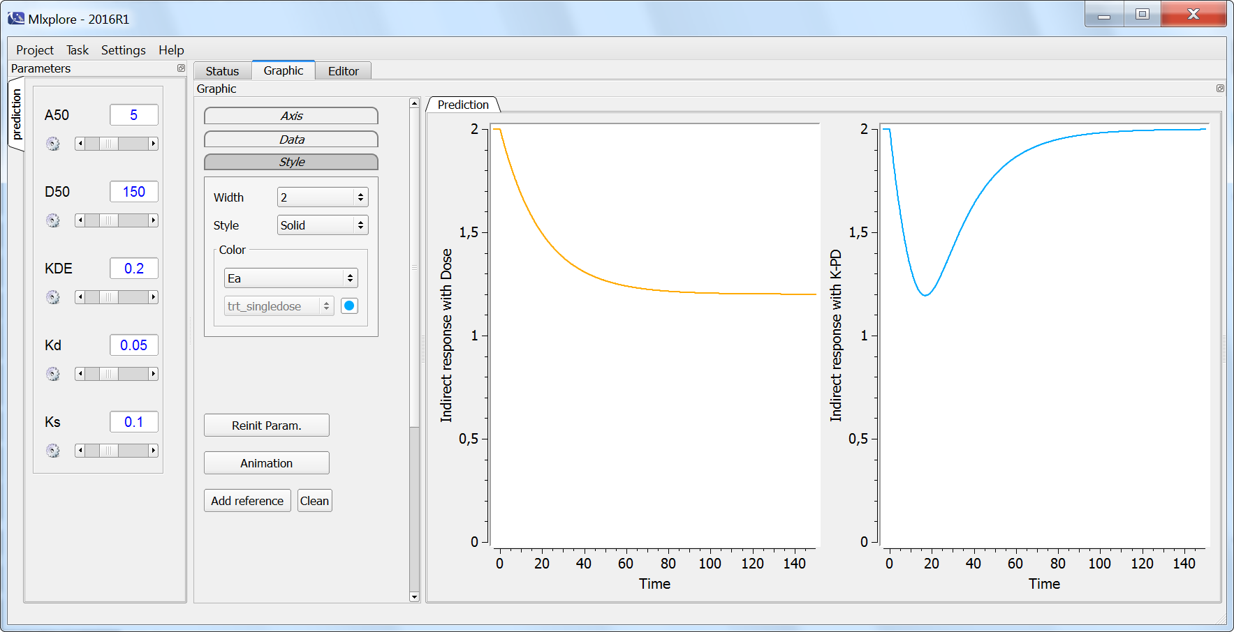
In the simulation below, the response of the dose-response model (orange) and of the K-PD model (blue) for a single dose are plotted. The two profiles differ clearly and only the K-PD model is able to capture the transient effect of the drug. If PD data is recorded densely after a dose, a K-PD is usually more appropriate to describe the data.

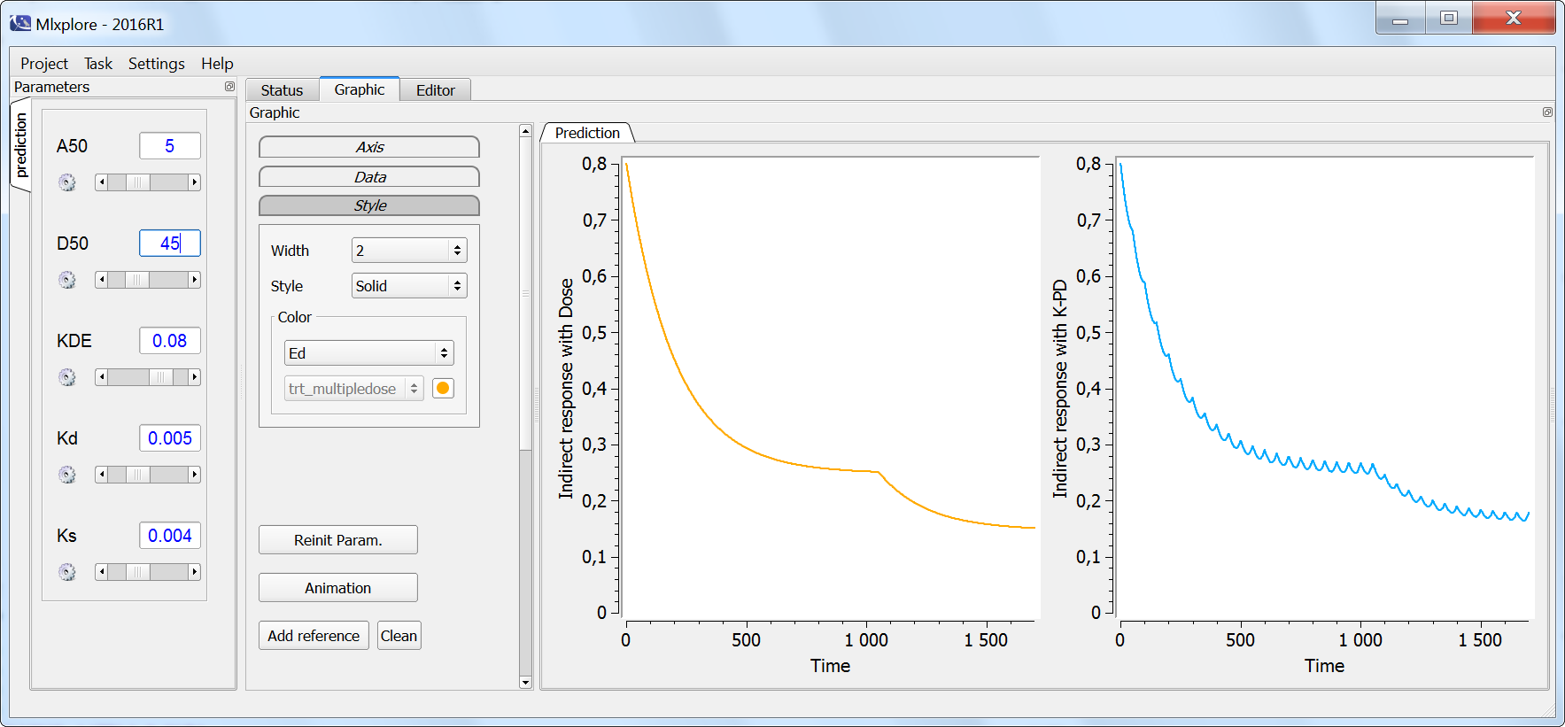
On the next simulation, the two models (dose-response in orange and K-PD in blue) are compared in the case of multiple doses. Note that at time 1000 the initial dose is increased by a factor 2. The only difference between the two models is that the K-PD model captures the small inter-dose variations, while the dose-response model does not. If the PD data is sparse, the dose-response model is usually sufficient. If the K-PD model is used, the KDE parameter may not be identifiable.

Data set formatting

The data set associated with K-PD models usually has one type of administration (administration of drug A) and one type of measurement (measurement of the response R). Below we show a data set extract:

The dose lines will be associated to the drug A via the depot statement depot(target=A). The measurement lines will be associated to the response R via the output statement output={R}. As there is only one type of administration and one type of observations, there is no need for the ADM and YTYPE columns.