When treatments span over a long time with numerous repeated doses, the clearance can be observed to change over time, for instance due to a change in the disease status. One possible approach to handle this case is to define in a parametric way how the clearance changes over time. A common assumption is to use an Imax or Emax model. Below, we show how to implement such a model in the Mlxtran language.
Examples of time-varying clearances are for instance presented for PEGylated Asparaginase, and for mycophenolic acid here
Mlxtran structural model
In the example below, we assume that the clearance is decreasing over time, with a sigmoidal shape. We consider a one-compartment model with first-order absorption. The Mlxtran code for the structural model reads:
[LONGITUDINAL]
input = {ka, V, Clini, Imax, gamma, T50}

PK:
depot(target=Ac, ka)

EQUATION:
t_0 = 0
Ac_0 = 0

Clapp = Clini * (1 - Imax * t^gamma/(t^gamma + T50^gamma))
ddt_Ac = - Clapp/V * Ac
Cc = Ac/V

OUTPUT:
output = {Cc}
The Clini parameter described the initial clearance, Imax the maximal reduction of clearance, T50 the time at which the clearance is reduced by half of the maximal reduction, and gamma characterizes the sigmoidal shape.
The apparent clearance Clapp is defined via an analytical formula depending on the time t and is then used in the ODE system. The first-order absorption is directly defined using the depot macro, which here indicates that the doses of the data set must be applied to the target Ac via a first-order absorption with rate ka (ka is a reserved keyword).
Model exploration with Mlxplore
To define an Mlxplore project, we in addition define the parameter values, the administration scheme and the output. The full code for the Mlxplore project reads:
<MODEL>
[LONGITUDINAL]
input = {ka, V, Cl, Imax, gamma, T50}

PK:
depot(target=Ac, ka)

EQUATION:
t_0 = 0
Ac_0 = 0

Clapp = Cl * (1 - Imax * t^gamma/(t^gamma + T50^gamma))
ddt_Ac = - Clapp/V * Ac
Cc = Ac/V

<PARAMETER>
ka=1
V=10
Cl = 10
Imax = 0.8
gamma=3
T50 = 50

<DESIGN>
[ADMINISTRATION]
adm = {time=0:10:300, amount=100}

<OUTPUT>
list={Cc}
grid=0.1:0.1:300
We decide to administrate the drug every 10 days during 300 days. The initial clearance is Clini=10 L/day and progressively decreases to Clend=Clini*(1-Imax)=2 L/day with a characteristic time of 50 days.
The simulation in Mlxplore shows how the peak and trough concentrations increase over time due to the reduced clearance: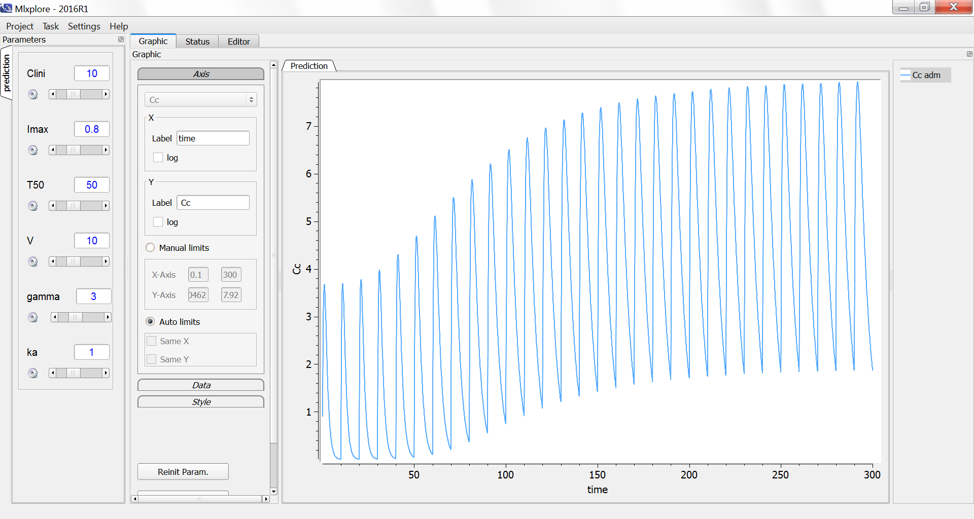
One can compare the original simulation (light blue) with a simulation where the clearance stays constant at 10 L/day (dark blue, with Imax=0):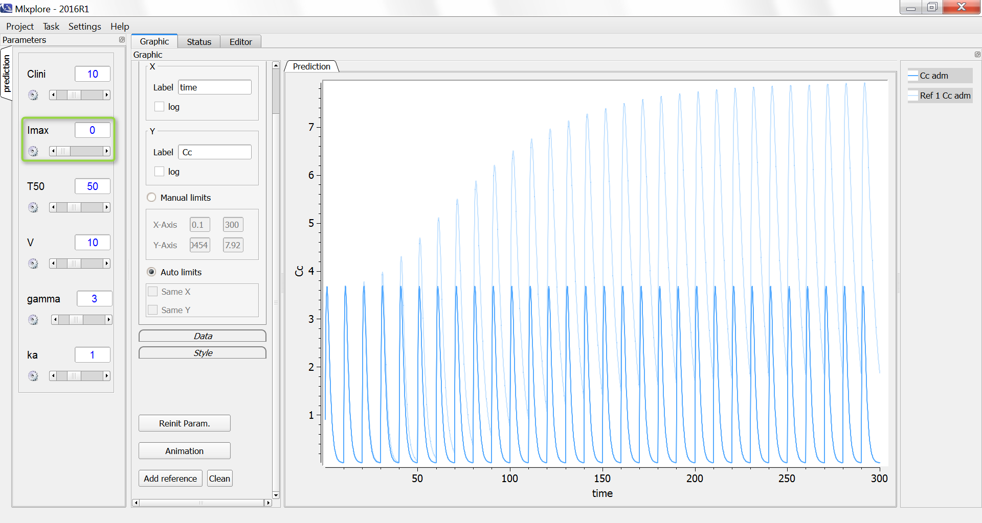
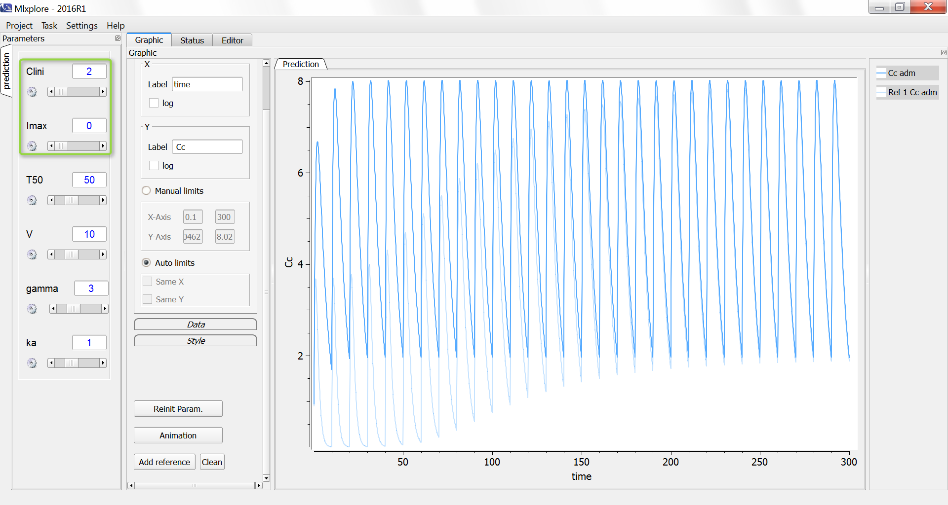
One can also compare the original simulation (light blue) with a simulation where the clearance stays constant at the Clend value 2 L/day (dark blue, with Imax=0 and Clini=2):