Absorption delays are common after oral administrations. They reflect the time needed for drug dissolution and/or for transit to the absorption site (Savic et al., 2007). Modeling these delays via a simple lag time may not properly capture the concentration-time profile and the progressive appearance of the drug to the absorption site. Mainly two approaches have been used to model these cases:
- transit compartment models, which describes the absorption as a multiple step process with a chain of presystemic compartments
- weibull absorptions, which describe the change in the absorption rate ka in a phenomenological way via a weibull function
test
Mlxtran code for transit compartments
Transit compartment can easily be implemented using the oral macro (when describing the model using macros) or the depot macro (when describing the model using ODEs), by adding the parameters Mtt and Ktr in addition to the usual absorption rate ka. Mtt represents the mean transit time and Ktr the transit rate between compartments. These two parameters are related via the number of compartments n:

Note: In case of multiple doses, the amounts in the depot, transit and absorption compartments are reset at each new doses. Thus the implementation is valid only if the dose is fully absorbed before the next dose administration. The amount in the central (and possibly other compartments) is not reset and can accumulate.
Example with model based on macros
[LONGITUDINAL]
input={ka, Mtt, Ktr, V, k}

PK:
compartment(cmt=1, volume=V, concentration=Cc)
oral(cmt=1, Mtt, Ktr, ka)
elimination(cmt=1,k)

OUTPUT:
output = Cc
Example with model based on ODEs
The entire absorption process is handled by the depot macro, which reads the dose information in the data set and applies an input rate to the target Ac corresponding to an oral administration with transit compartments.
[LONGITUDINAL]
input={ka, Mtt, Ktr, V, k}

PK:
depot(target=Ac, ka, Mtt, Ktr)

EQUATION:
t_0 = 0
Ac_0 = 0

ddt_Ac = - k * Ac
Cc = Ac/V

OUTPUT:
output = Cc
Mlxtran code for Weibull absorptions
Despite the lack of physiological basis, the Weibull model is appreciated for its flexibility (Zhou et al, 2003). We here demonstrate the implementation of one Weibull function models. The extension to two Weibull functions is straightforward. The time-varying absorption rate is:
$$k_a(t) = \frac{\beta}{\alpha}\left( \frac{t}{\alpha} \right) ^{\beta – 1}$$
The model requires to be written as an ODE system with a depot compartment and at last a central compartment. The transfer of matter from the depot compartment to the central compartment is described using a time-varying rate constant. To allow for multiple doses, the time is calculated with respect to the time of the last dose, using the tDose keyword. Note that only one type of administration (only oral or only iv for instance) is allowed per individual, as the tDose keyword doesn’t distinguish between different administration types ADM.
The alpha parameter describes the delay, while the beta parameter influences the steepness of the absorption phase.
[LONGITUDINAL]
input={beta, alpha, V, k}

PK:
depot(target=Ad)

EQUATION:
t_0 = 0
Ad_0 = 0
Ac_0 = 0

ddt_Ad = -Ad * (beta/alpha)*(max(0,t-tDose)/alpha)^(beta-1)
ddt_Ac = Ad * (beta/alpha)*(max(0,t-tDose)/alpha)^(beta-1) - k*Ac
Cc = Ac/V

OUTPUT:
output = Cc
Exploration with Mlxplore
We first note that the transit compartment model has 3 parameters for the absorption (Mtt, Ktr, ka) while the Weibull model has two (alpha, beta). If the transit compartment model appears overparameterized, the ka rate can be set to be equal to Ktr via oral(cmt=1, Mtt, Ktr, ka=Ktr).
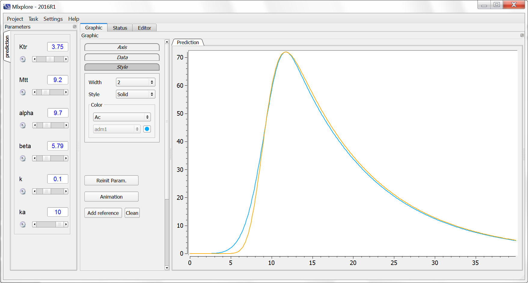
Let compare the behavior of these two models using Mlxplore. The Mlxplore code reads:
<MODEL>
[LONGITUDINAL]
input={beta, alpha, ka, Mtt, Ktr, k}

PK:
depot(target=Ad)

compartment(cmt=1,amount=At)
absorption(cmt=1, Mtt, Ktr, ka)
elimination(cmt=1,k)

EQUATION:
t_0 = 0
Ad_0 = 0
Ac_0 = 0

ddt_Ad = -Ad * (beta/alpha)*(max(0,t-tDose)/alpha)^(beta-1)
ddt_Ac = Ad * (beta/alpha)*(max(0,t-tDose)/alpha)^(beta-1) - k *Ac

<PARAMETER>
beta= 6
alpha = 10
ka = 3
Mtt = 10
Ktr = 3
k = 0.1

<DESIGN>
[ADMINISTRATION]
adm1 = {time = {0}, amount=100, type=1}

<OUTPUT>
list={Ac,At}
grid=0:0.1:40

<RESULTS>
[GRAPHICS]
p1 = {y={Ac,At}}
The simulated amount for the weibull absorption (blue) and the transit compartments (orange) are similar, with the transit compartment model allowing for some more flexibility thank to the additional parameter.
