We here present the system of equation corresponding to the constant Rtot TMDD model, as well as the model behavior.
Equations
If the degradation rates of the free receptor and the complex are similar (i.e the binding of the ligand to the receptor does not modify the receptor internalization rate), it may not be possible to identify both of them. If both rates are equal (
=R_0=\frac{k_{\textrm{syn}}}{k_{\textrm{deg}}}")
}{V} - (k_{\textrm{el}}+k_{\textrm{on}}R_0) \: L + (k_{\textrm{off}}+k_{\textrm{on}}L)\:P \\ \dfrac{dP}{dt} &=& k_{\textrm{on}}\:R_0\:L - (k_{\textrm{off}} + k_{\textrm{int}} + k_{\textrm{on}}L)\:P \end{array}")
with L the concentration of the ligand in plasma and P the concentration of the complex. V is the volume of the central compartment for the ligand, kel the linear elimination rate for the ligand, kon the binding rate, koff the dissociation rate, R0 the initial receptor concentration, and kint the degradation rate of the complex. In(t) represents the input function, corresponding to the input rate (amount per unit time) of the ligand into the central compartment due to the ligand administration.
In the library model file, a slightly different parameterization is used using 
The free receptor concentration can be calculated via 
With 2 compartments for the free ligand, one obtains:
}{V} - (k_{\textrm{el}}+k_{\textrm{on}}R_0) \: L + (k_{\textrm{off}}+k_{\textrm{on}}L)\:P - k_{\textrm{12}}\:L + k_{\textrm{21}}\:A/V \\ \dfrac{dP}{dt} &=& k_{\textrm{on}}\:R_0\:L - (k_{\textrm{off}} + k_{\textrm{int}} + k_{\textrm{on}}L)\:P \\ \dfrac{dA}{dt} &=& k_{\textrm{12}}\:L\:V - k_{\textrm{21}}\:A \end{array}")
with A the amount of ligand in peripheral tissues, k12 the rate of transfert from central to peripheral, and k21 the rate in the opposite direction.
Model properties
We investigate the influence of each parameter on the typical free ligand concentration-time shape for several dose amounts (bolus administration).
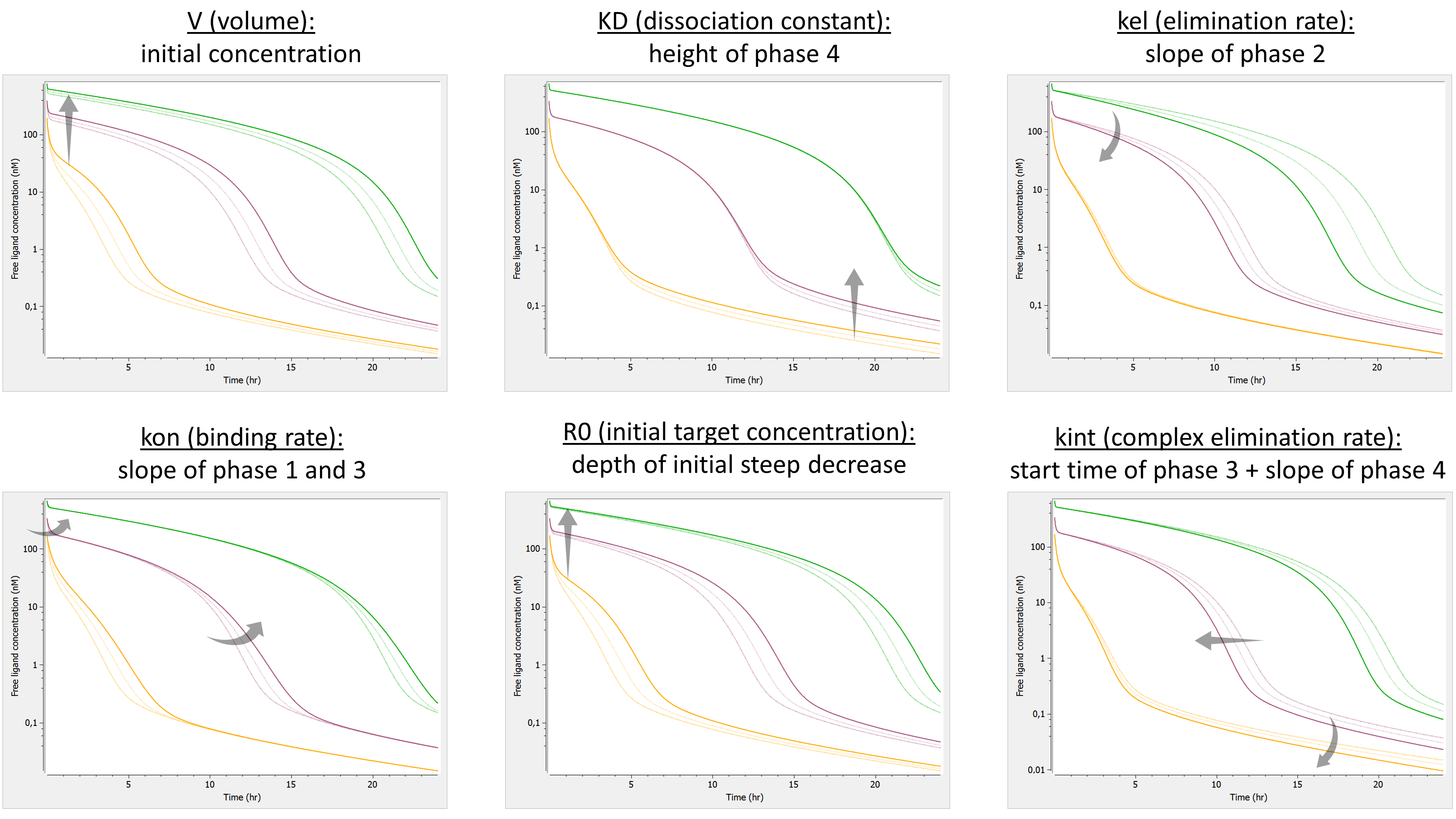
The summary figure is the following:
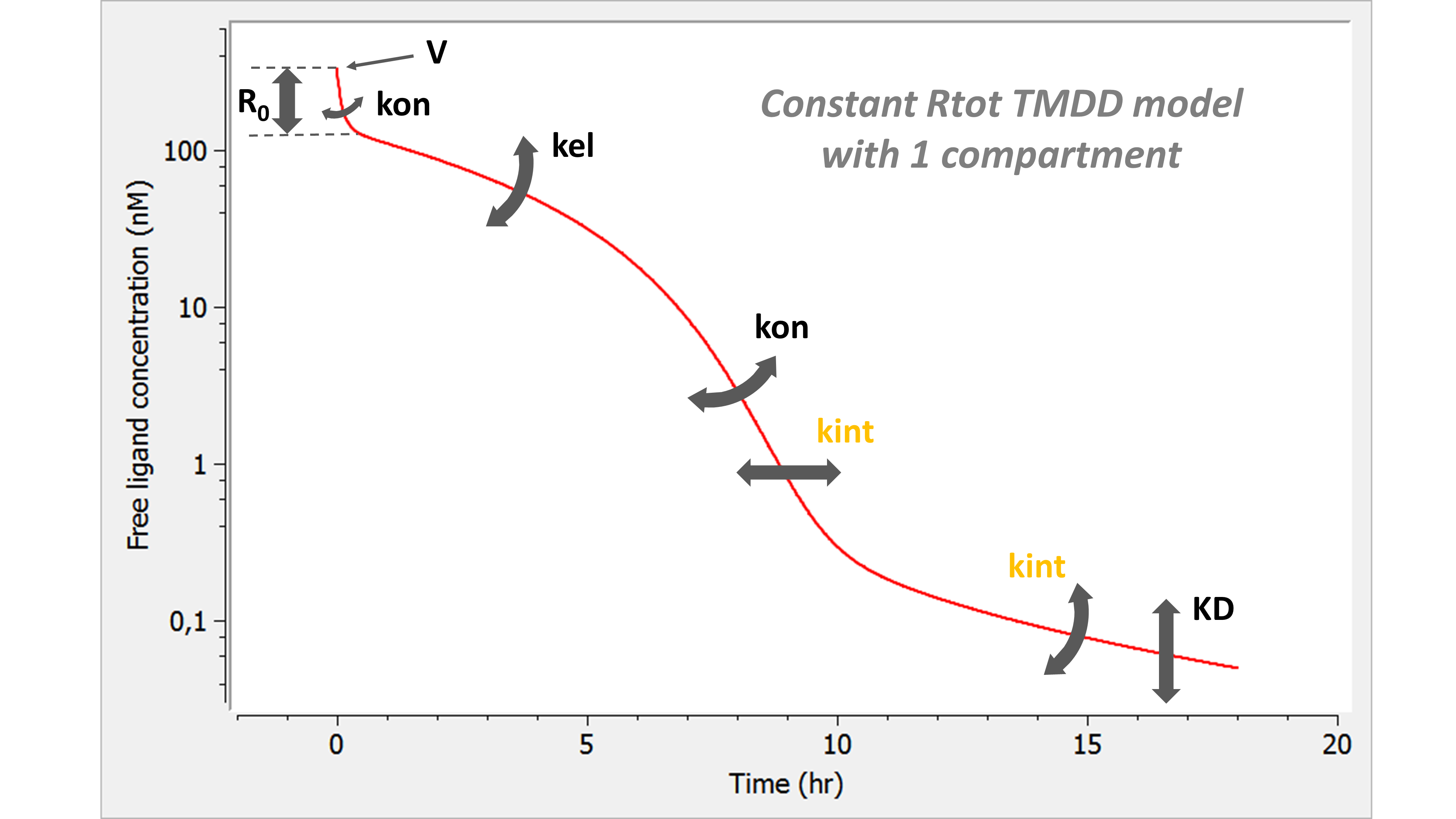
On opposite to the QE/QSS models, the constant Rtot model still captures all four phases of the free ligand concentration-time curve. However, note that because 
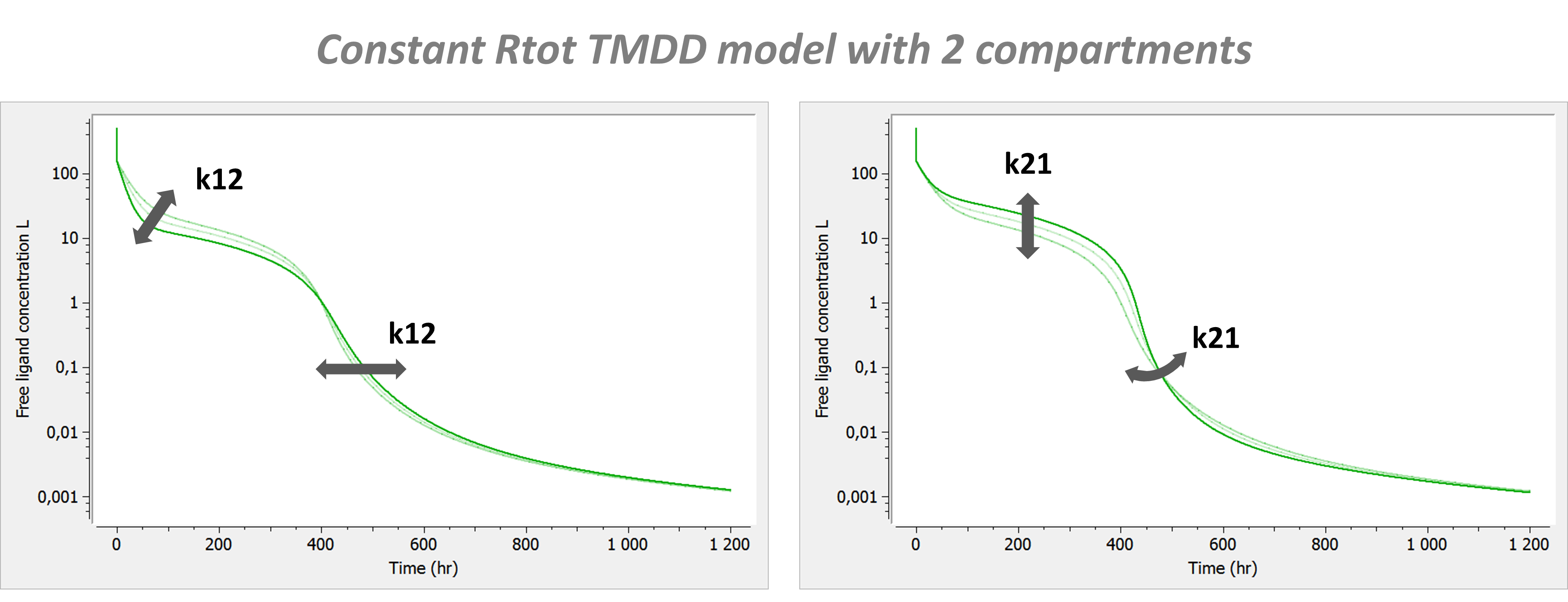
Model with 2 compartments
If a second compartment is added, the shape is modified in the following way. Note that kon has been chosen large (very steep phase 1), to better focus on phase 2, where k12 and k21 have their main effect.
Click here to go back to main TMDD page.