This page presents the TTE model library proposed by Lixoft. It includes an introduction on time-to-event data, the different ways to model this kind of data, and typical parametric models.
|
|
What is time-to-event data
In case of time-to-event data the recorded observations are the times at which events occur. We can for instance record the time (duration) from diagnosis of a disease until death, or the time between administration of a drug and the next epileptic seizures. In the first case, the event is one-off, while in the second it can be repeated.
In addition, the event can be:
- exactly observed: we know the event has happen exactly at time \(t_i (T_i=t_i)\)
- interval censored: we know the event has happen during a time interval, but not exactly when \((a_i \leq T_i \leq b_i)\)
- right censored: the observation period ends before the event can be observed \((T_i > t_{end}) \)
Formatting of time-to-event data in the MonolixSuite
In the data set, exactly observed events, interval censored events and right censoring are recorded for each individual. Contrary to other softwares for survival analysis, the MonolixSuite requires to specify the time at which the observation period starts. This allow to define the data set using absolute times, in addition to durations (if the start time is zero, the records represent durations between the start time and the event). 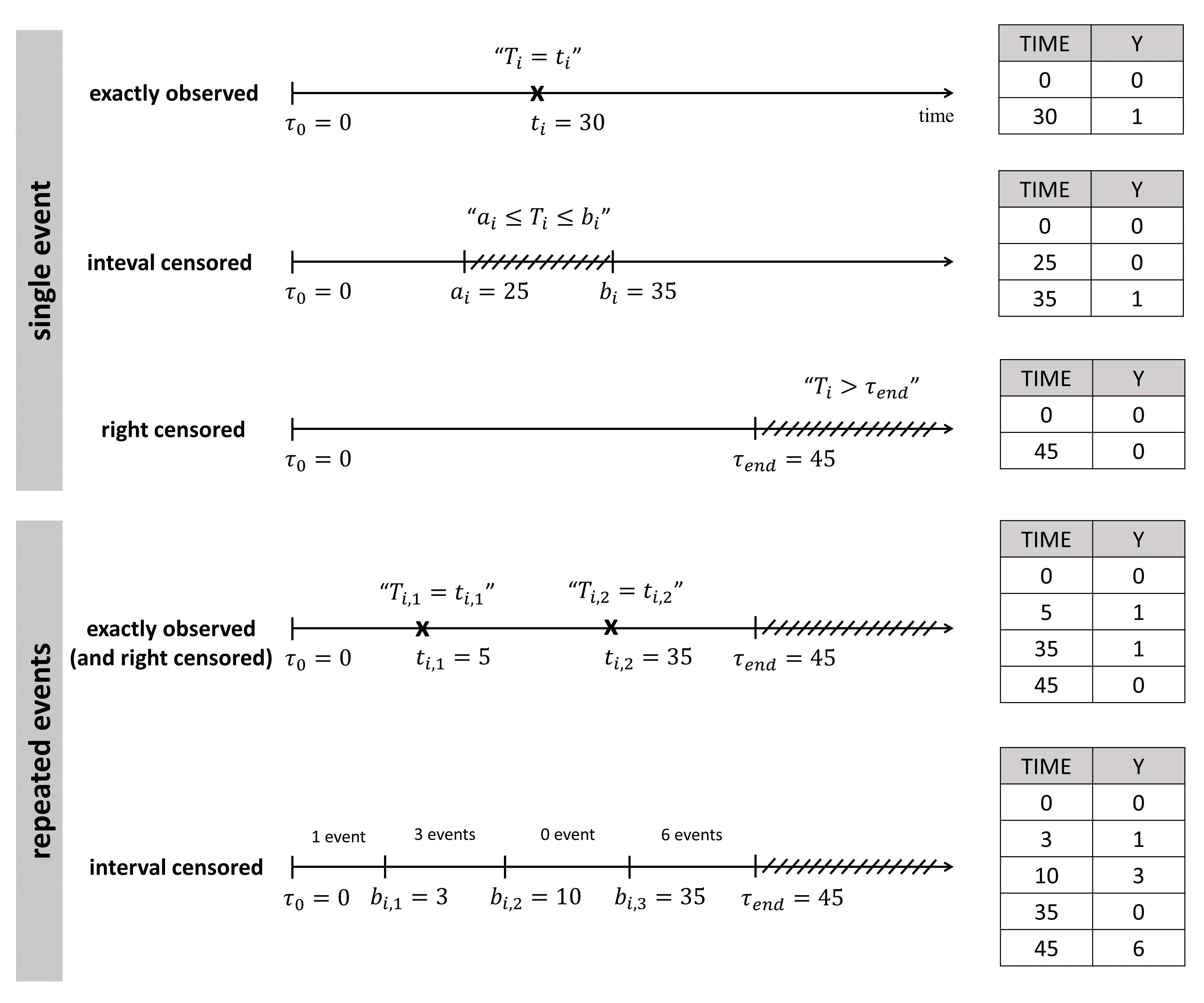
For instance for single events, exactly observed (with or without right censoring), one must indicate the start time of the observation period (Y=0), and the time of event (Y=1) or the time of the end of the observation period if no event has occurred (Y=0). In the following example:
ID TIME Y
1   0   0
1  34   1
2   0   0
2  80   0
the observation period last from starting time t=0 to the final time t=80. For individual 1, the event is observed at t=34, and for individual 2, no event is observed during the period. Thus it is indicated that at the final time (t=80), no event had occurred. Using absolute times instead of durations, we could equivalently write:
ID TIME Y
1  20   0
1  54   1
2  33   0
2  113  0
The durations between start time and event (or end of the observation period) are the same as before, but this time we record the day at which the patients enter the study and the days at which they have events or leave the study. Different patients may enter the study at different times.
Important concepts: hazard and survival
Two functions have a key role in time-to-event analysis: the survival function and the hazard function. The survival function S(t) is the probability that the event happens after time t. A common way to estimate it non-parametrically is to calculate the Kaplan-Meier estimate. The hazard function h(t) is the instantaneous rate of an event, given that it has not already occurred. Both are linked by the following equation:
$$S(t)=e^{-\int_0^t h(x) dx}$$
Different types of approaches
Depending on the goal of the time-to-event analysis, different modeling approaches can be used: non-parametric, semi-parametric (Cox models) and parametric.
- Non-parametric models do not require assumptions on the shape of the hazard or survival. Using the Kaplan-Meier estimate, statistical tests can be performed to check if the survival differs between sub-populations. The main limitations of this approach are that (i) only categorical covariates can be tested and (ii) the way the survival is affected by the covariate cannot be assessed.
- Semi-parametric models (Cox models) assume that the hazard can be written as a baseline hazard (that depends only on time), multiplied by a term that depends only on the covariates (and not time). Under this hypothesis of proportional covariate effect, one can analyze the effect of covariates (categorical and continuous) in a parametric way, leaving the baseline hazard undefined.
- Parametric models require to fully specify the hazard function. If a good model can be found, statistical tests are more powerful than for semi-parametric models. In addition, there is no restrictions on how the covariates affects the hazard. Parametric models can also be easily used for predictions.
The table below synthesizes the possibilities for the 3 approaches.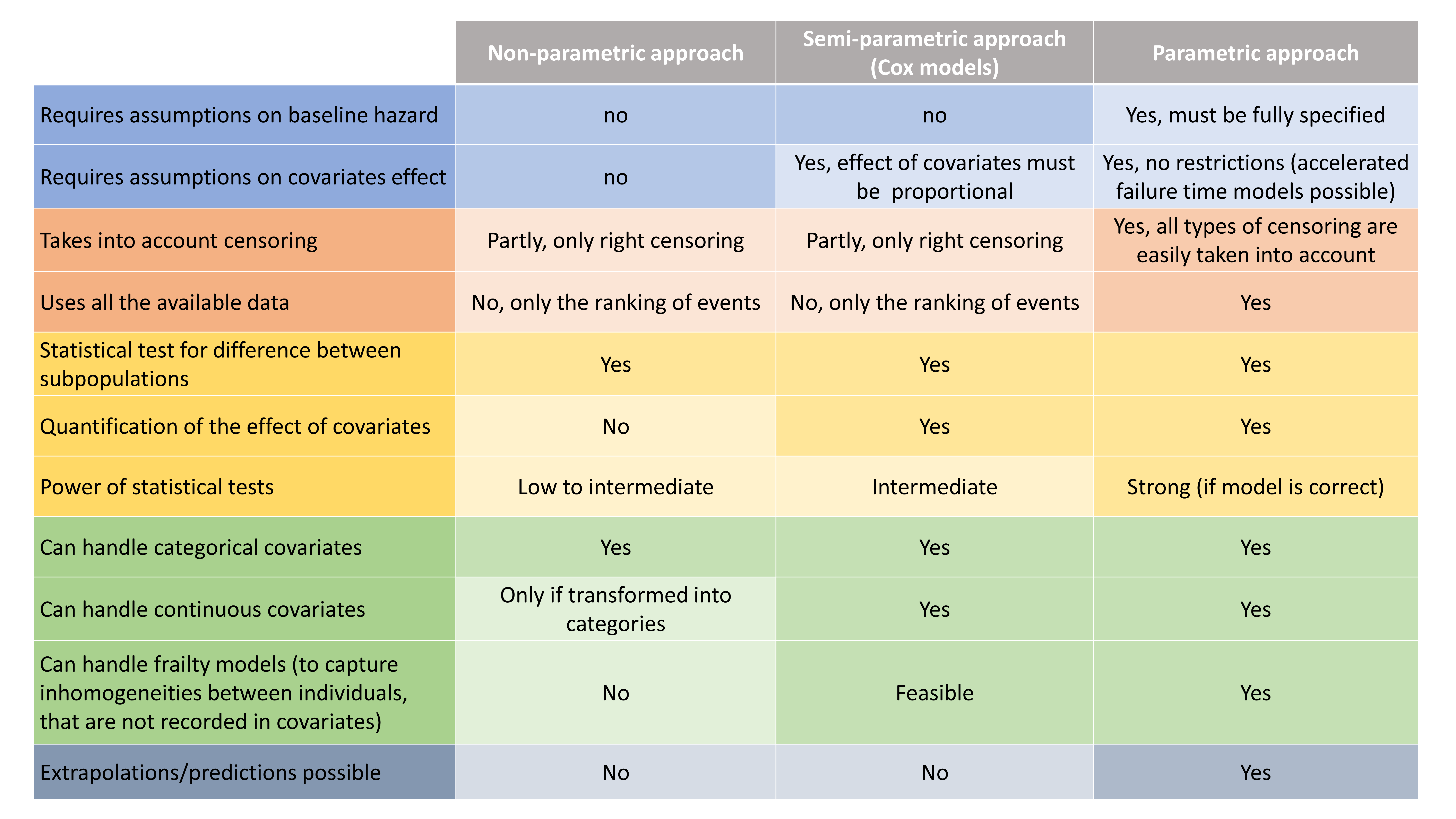
Focus on parametric modeling with the MonolixSuite
In the MonolixSuite, the only possible approach is the parametric approach. The model is defined via the hazard function, which in a population approach typically depends on individual parameters: \(h(t,\psi_i)\). With the hazard function, the survival function can easily be computed, as well as the conditional distribution \(p_{y_i|\psi_i}\) for various censoring situations (which is required for parameter estimation via SAEM, log-likelihood calculation, etc).
The typical syntax to define the output is the following:
DEFINITION:
Event = {type=event, maxEventNumber=1, hazard=h}
The output Event will be matched to the time-to-event data of the data set. The hazard function h is usually defined via an expression including the input individual parameters. For one-off events, the maximal number of events per individual is 1. It is important to indicate it in the maxEventNumber argument to speed up calculations. To use the model for simulations with Simulx, rightCensoringTime must be given as additional argument. Check here for details.
Note that the hazard can be a function of other variables such as drug concentration or tumor burden for instance (joint PK-TTE or PD-TTE models). An example of the syntax is given here.
Library of parametric models for time-to-event data
To describe the various shapes that the survival Kaplan-Meier estimate can take, several hazard functions have been proposed. Below we display the survival curves, for the most typical hazard functions:
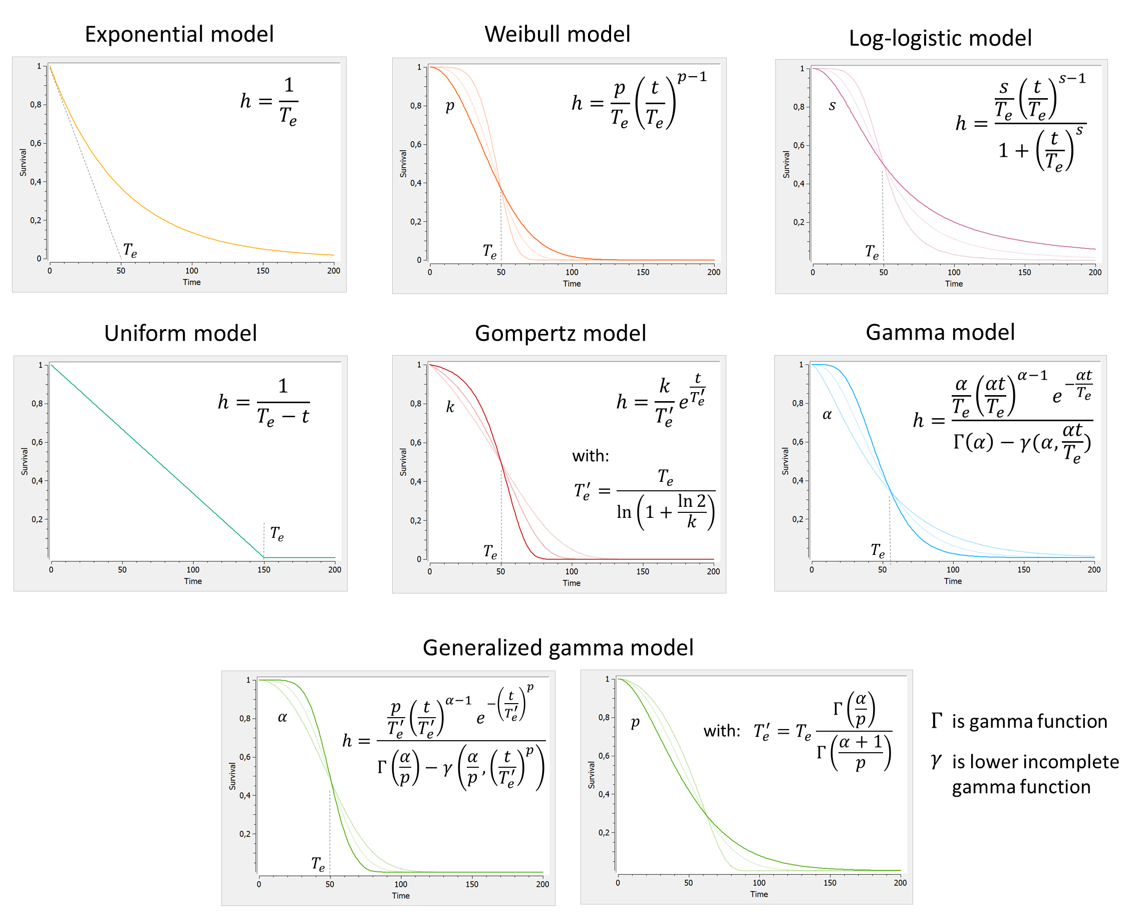
A few comments:
- We have reparametrized \(T_e’\) as a function of \(T_e\) to better separate the effects of the scale parameter (characteristic time) and the shape parameter (shape of the curve).
- All parameters are positive. If we assume inter-individual variability, a log-normal distribution is usually appropriate.
The table below summarizes the number of parameters and typical parameter values: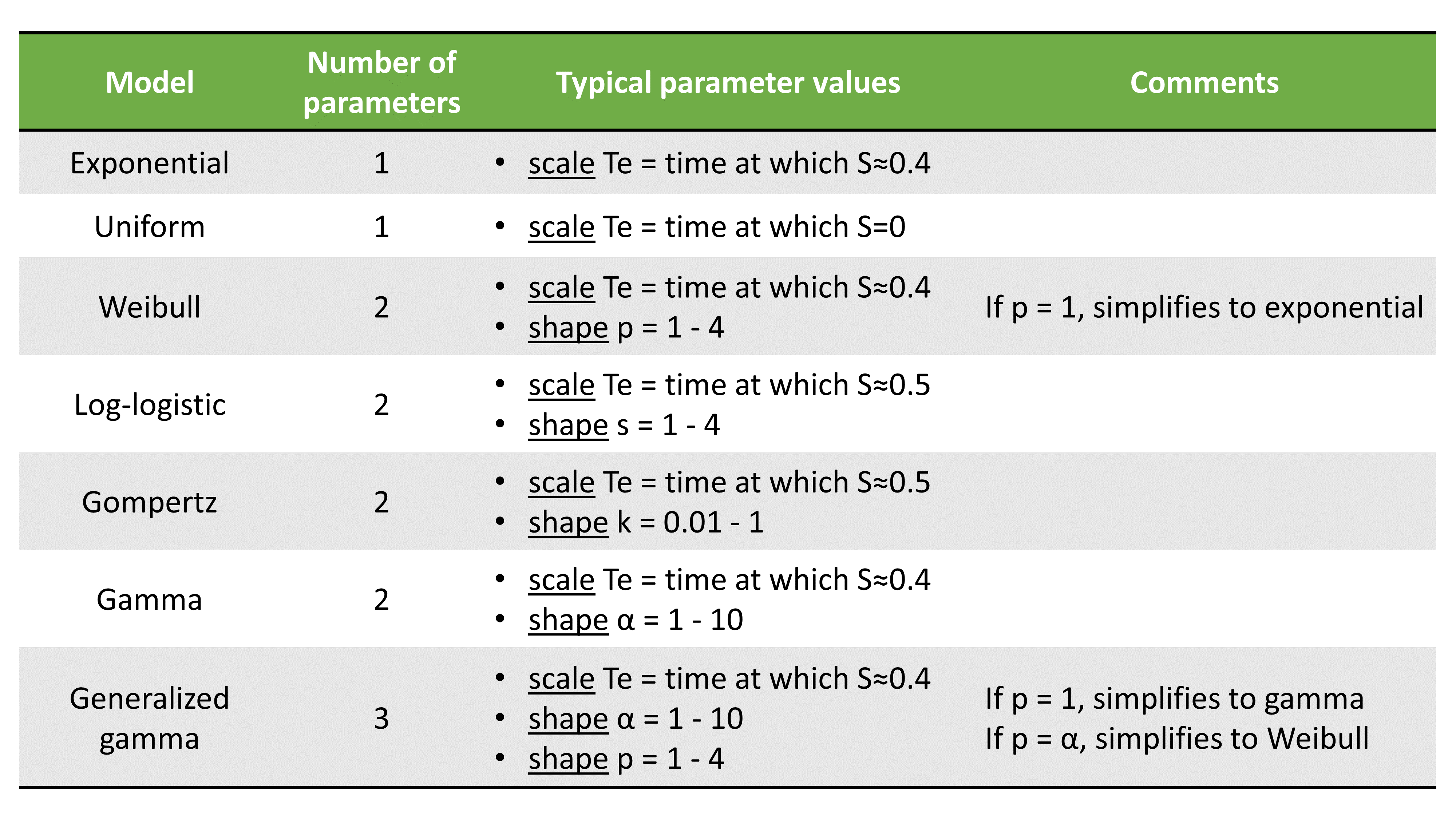
For each model, we can in addition consider a delay del as additional parameter. The delay will simply shift the survival curve to the right (later times). For t<del, the survival is S(t<del)=1.
Downloads:
These models can be explore in Mlxplore (download Mlxplore project here). A shiny-mlxR app also permits to give any hazard function and visualize the corresponding survival curve (click here).
All models are available as Mlxtran model file in the TTE library. Each model can be with/without delay and for single/repeated events. For performance reasons, it is important to choose the file ending with ‘_singleEvent.txt’ if you want to model one-off events (death, drop-out, etc).
Case studies
Two case studies show the modeling and simulation workflow for TTE data: