We here present the system of equation corresponding to the Wagner TMDD model, as well as the model behavior.
Equations
The constant Rtot, QSS/QE and irreversible binding approximations may still be overparametrized. A further simplification can be made and is called the Wagner model. It has initially been described in Biopharmaceutics and relevant pharmacokinetics by Wagner. The Wagner model can be derived from the QE/QSS approximation assuming in addition that the total receptor pool is constant (i.e 


Two formulations are possible, either using the free ligand concentration L or using the total ligand concentration Ltot. To our knowledge, the formulation using L is always presented:
}{V} - k_{\textrm{el}} \: L - \frac{R_0k_{\textrm{int}}L}{K_D+L} }{1+\frac{R_0K_D}{(K_D+L)^2}}")
with L the concentration of the ligand in plasma. V is the volume of the central compartment for the ligand, kel the linear elimination rate for the ligand, KD the dissociation constant, R0 the initial receptor concentration, and kint the degradation rate of the complex. In(t) represents the input function, corresponding to the input rate (amount per unit time) of the ligand into the central compartment due to the ligand administration.
If the system is derived from the QSS approximation, then KD is replaced by KSS. If it is derived from the irreversible model, then KD is replaced by 
This formulation presents a disadvantage: in case of a bolus administration, the initial free ligand concentration cannot be assumed to be 
however, the situation becomes more complicated for subsequent doses, where Rtot(t) must be used instead of Rtot(t=0)=R0.
![L(t=0)=\frac{1}{2}\left[ (\frac{D}{V}-R_0-K_{D})+\sqrt{(\frac{D}{V}-R_0-K_{D})^2+4K_{D}\frac{D}{V}}\right]](http://s0.wp.com/latex.php?latex=L%28t%3D0%29%3D%5Cfrac%7B1%7D%7B2%7D%5Cleft%5B+%28%5Cfrac%7BD%7D%7BV%7D-R_0-K_%7BD%7D%29%2B%5Csqrt%7B%28%5Cfrac%7BD%7D%7BV%7D-R_0-K_%7BD%7D%29%5E2%2B4K_%7BD%7D%5Cfrac%7BD%7D%7BV%7D%7D%5Cright%5D+&bg=ffffff&fg=000&s=0.5 "L(t=0)=\frac{1}{2}\left[ (\frac{D}{V}-R_0-K_{D})+\sqrt{(\frac{D}{V}-R_0-K_{D})^2+4K_{D}\frac{D}{V}}\right]")
We thus propose to use instead the formulation in Ltot (total ligand concentration):
![\begin{array}{ccl} \dfrac{dL_{\textrm{tot}}}{dt} &=& \dfrac{\textrm{In}(t)}{V} - k_{\textrm{int}} \: L_{\textrm{tot}} - (k_{\textrm{el}}-k_{\textrm{int}})L \\ L&=&\frac{1}{2}\left[ (L_{\textrm{tot}}-R_0-K_D)+\sqrt{(L_{\textrm{tot}}-R_0-K_D)^2+4K_DL_{\textrm{tot}}}\right] \end{array}](http://s0.wp.com/latex.php?latex=%5Cbegin%7Barray%7D%7Bccl%7D%C2%A0%5Cdfrac%7BdL_%7B%5Ctextrm%7Btot%7D%7D%7D%7Bdt%7D+%26%3D%26+%5Cdfrac%7B%5Ctextrm%7BIn%7D%28t%29%7D%7BV%7D+-+k_%7B%5Ctextrm%7Bint%7D%7D+%5C%3A%C2%A0L_%7B%5Ctextrm%7Btot%7D%7D+-+%28k_%7B%5Ctextrm%7Bel%7D%7D-k_%7B%5Ctextrm%7Bint%7D%7D%29L+%C2%A0+%5C%5C+L%26%3D%26%5Cfrac%7B1%7D%7B2%7D%5Cleft%5B+%28L_%7B%5Ctextrm%7Btot%7D%7D-R_0-K_D%29%2B%5Csqrt%7B%28L_%7B%5Ctextrm%7Btot%7D%7D-R_0-K_D%29%5E2%2B4K_DL_%7B%5Ctextrm%7Btot%7D%7D%7D%5Cright%5D+%5Cend%7Barray%7D&bg=ffffff&fg=000&s=0.5 "\begin{array}{ccl} \dfrac{dL_{\textrm{tot}}}{dt} &=& \dfrac{\textrm{In}(t)}{V} - k_{\textrm{int}} \: L_{\textrm{tot}} - (k_{\textrm{el}}-k_{\textrm{int}})L \\ L&=&\frac{1}{2}\left[ (L_{\textrm{tot}}-R_0-K_D)+\sqrt{(L_{\textrm{tot}}-R_0-K_D)^2+4K_DL_{\textrm{tot}}}\right] \end{array}")
The number of parameters is the same, and the system complexity also. P, R and Rtot can easily be calculated using 

")
=\frac{D}{V}=P(t=0)+L(t=0)")
With a second compartment, the system becomes:
![\begin{array}{ccl} \dfrac{dL_{\textrm{tot}}}{dt} &=& \dfrac{\textrm{In}(t)}{V} - k_{\textrm{int}} \: L_{\textrm{tot}} - (k_{\textrm{el}}-k_{\textrm{int}})L - k_{\textrm{12}}\:L + k_{\textrm{21}}\:A/V \\ \dfrac{dA}{dt} &=& k_{\textrm{12}}\:L\:V - k_{\textrm{21}}\:A \\ L&=&\frac{1}{2}\left[ (L_{\textrm{tot}}-R_0-K_D)+\sqrt{(L_{\textrm{tot}}-R_0-K_D)^2+4K_DL_{\textrm{tot}}}\right] \end{array}](http://s0.wp.com/latex.php?latex=%5Cbegin%7Barray%7D%7Bccl%7D%C2%A0%5Cdfrac%7BdL_%7B%5Ctextrm%7Btot%7D%7D%7D%7Bdt%7D+%26%3D%26+%5Cdfrac%7B%5Ctextrm%7BIn%7D%28t%29%7D%7BV%7D+-+k_%7B%5Ctextrm%7Bint%7D%7D+%5C%3A%C2%A0L_%7B%5Ctextrm%7Btot%7D%7D+-+%28k_%7B%5Ctextrm%7Bel%7D%7D-k_%7B%5Ctextrm%7Bint%7D%7D%29L+-+k_%7B%5Ctextrm%7B12%7D%7D%5C%3AL+%2B+k_%7B%5Ctextrm%7B21%7D%7D%5C%3AA%2FV+%5C%5C+%5Cdfrac%7BdA%7D%7Bdt%7D+%26%3D%26%C2%A0k_%7B%5Ctextrm%7B12%7D%7D%5C%3AL%5C%3AV+-+k_%7B%5Ctextrm%7B21%7D%7D%5C%3AA+%C2%A0%5C%5C+L%26%3D%26%5Cfrac%7B1%7D%7B2%7D%5Cleft%5B+%28L_%7B%5Ctextrm%7Btot%7D%7D-R_0-K_D%29%2B%5Csqrt%7B%28L_%7B%5Ctextrm%7Btot%7D%7D-R_0-K_D%29%5E2%2B4K_DL_%7B%5Ctextrm%7Btot%7D%7D%7D%5Cright%5D+%5Cend%7Barray%7D&bg=ffffff&fg=000&s=0.5 "\begin{array}{ccl} \dfrac{dL_{\textrm{tot}}}{dt} &=& \dfrac{\textrm{In}(t)}{V} - k_{\textrm{int}} \: L_{\textrm{tot}} - (k_{\textrm{el}}-k_{\textrm{int}})L - k_{\textrm{12}}\:L + k_{\textrm{21}}\:A/V \\ \dfrac{dA}{dt} &=& k_{\textrm{12}}\:L\:V - k_{\textrm{21}}\:A \\ L&=&\frac{1}{2}\left[ (L_{\textrm{tot}}-R_0-K_D)+\sqrt{(L_{\textrm{tot}}-R_0-K_D)^2+4K_DL_{\textrm{tot}}}\right] \end{array}")
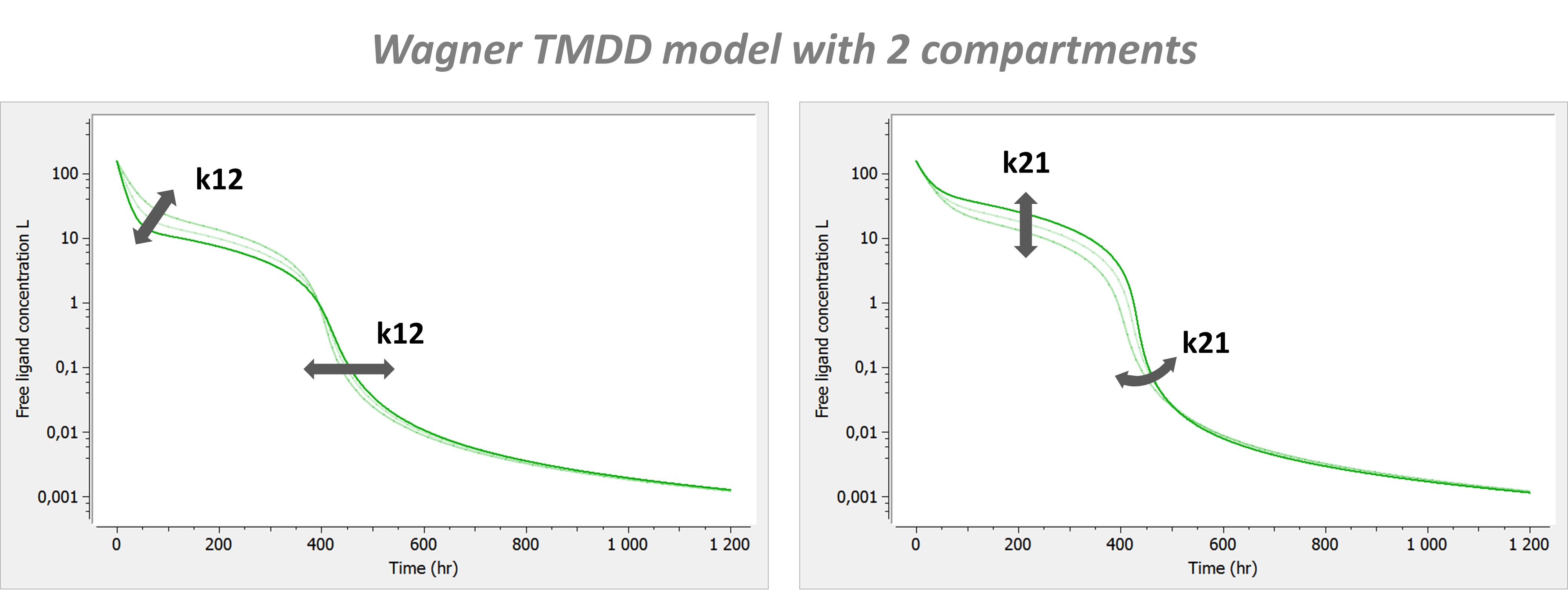
with A the amount of ligand in peripheral tissues, k12 the rate of transfert from central to peripheral, and k21 the rate in the opposite direction.
Model properties
We investigate the influence of each parameter on the typical free ligand concentration-time shape for several dose amounts (bolus administration).

The summary picture is:
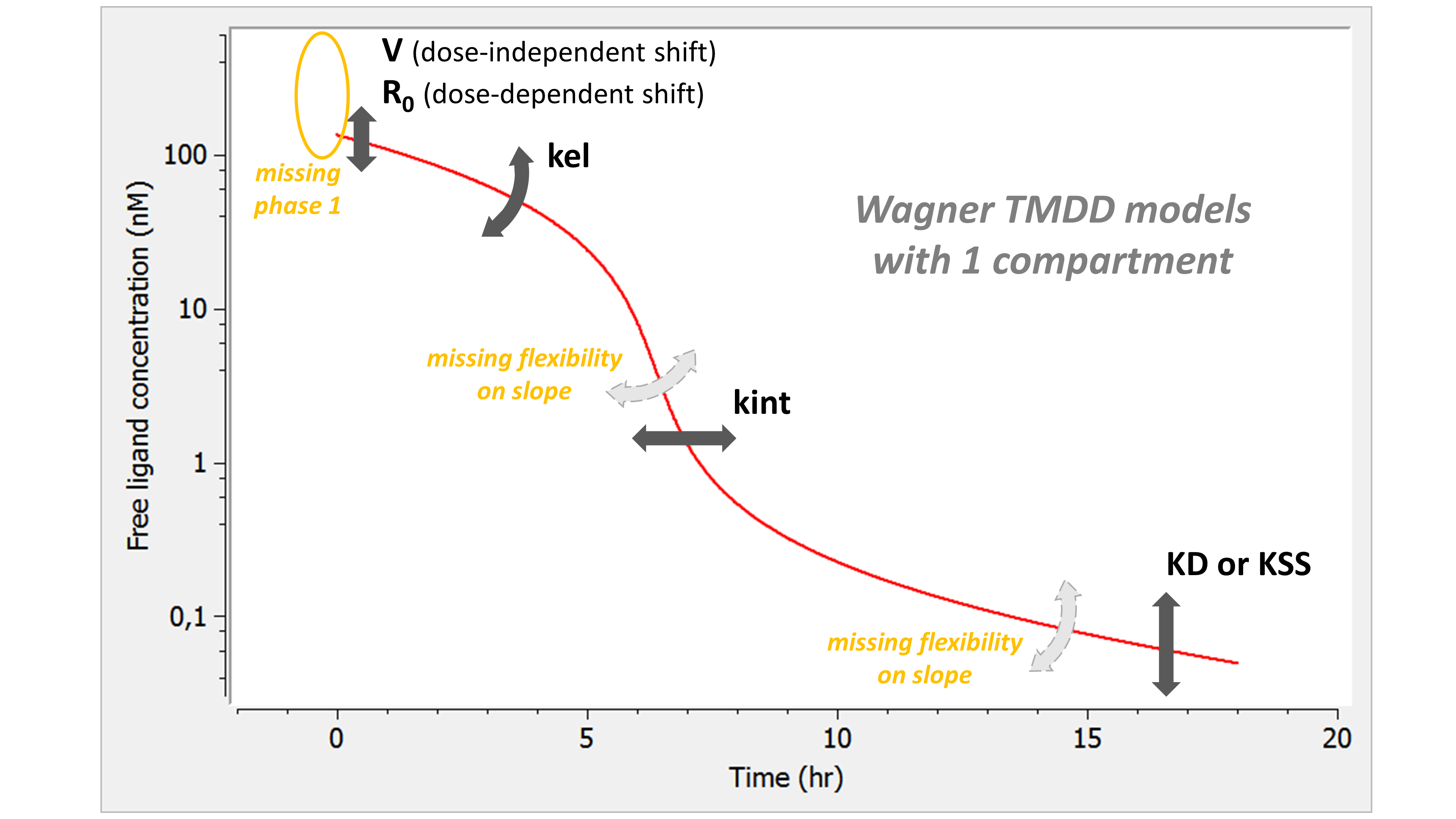
The Wagner model combines the assumptions of the QE (or QSS) model and those of the constant Rtot model. As for QE, the phase 1 is missing: the free concentration of ligand directly starts at the equilibrium concentration. In addition, the lack of kon passes on the lack of flexibility in the slope of phase 3. As for the constant Rtot model, we also have a lack of flexibility on the slope of phase 4.
Model with 2 compartments
If a second compartment is added, the shape is modified in the following way.
Click here to go back to main TMDD page.