PK/PD model with indirect response

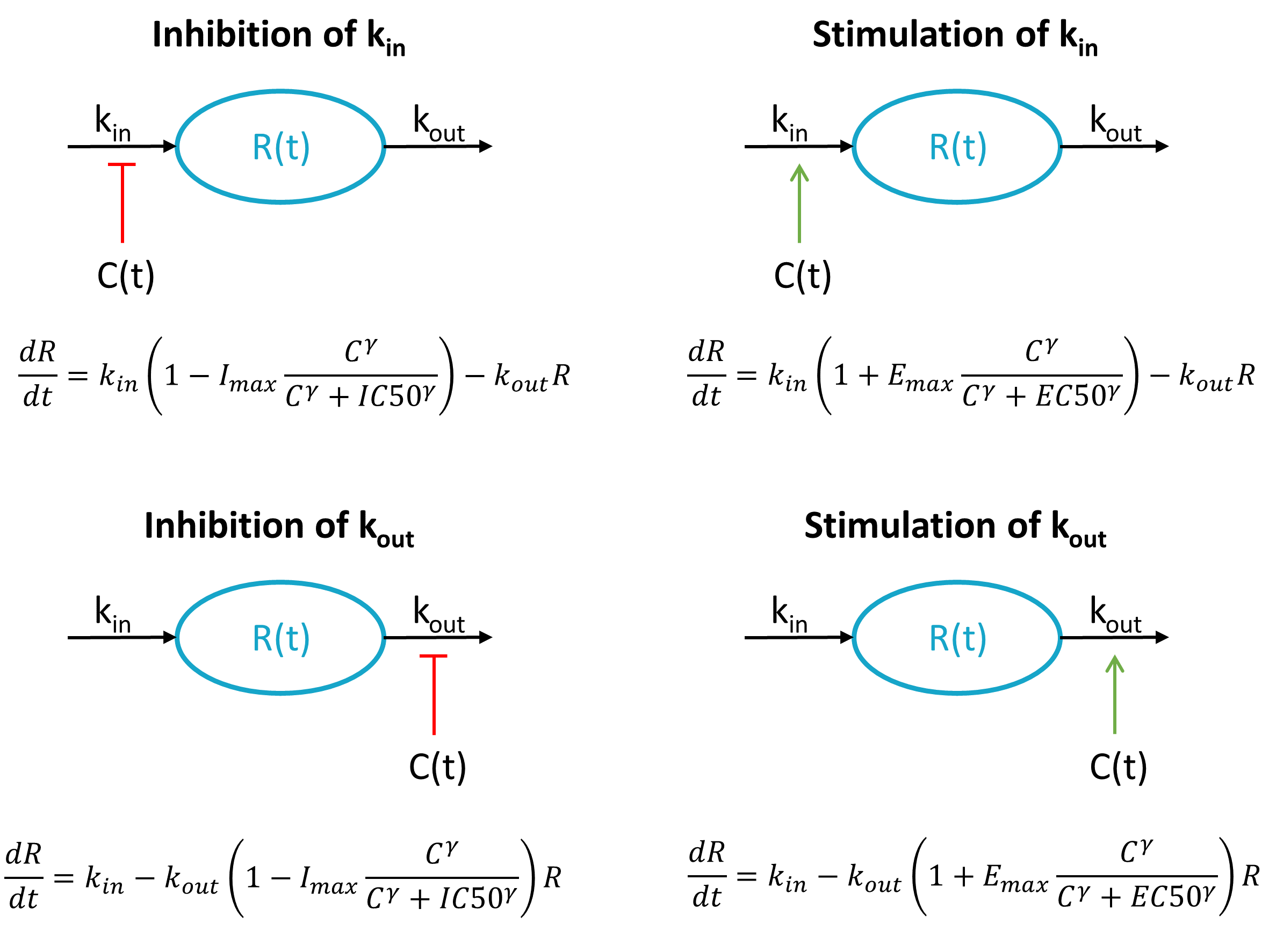
When the response to a drug is not directly related to the drug’s concentration (or to the concentration in a effect compartment), indirect response models have been proposed. The response R is assumed to be produced by a zero-order synthesis rate and degraded via a first-order process:

$\frac{dR}{dt}=k_{in}-k_{out}R$

The baseline response is $R_0=\frac{k_{in}}{k_{out}}$ .

The drug can act on kin or kout by inhibition or stimulation, leading to 4 situations:

Each of these 4 cases have been presented and analysed in Dayneka et al. (1993).

Mlxtran models

Below we present the mlxtran code for each situation, in the case of a bolus administration of the drug and one compartment. The PK part of the model can easily be modified to represent more complex pharmacokinetics.

We here assume that both the drug concentration (tagged with YTYPE=1 in the data set) and the response (tagged with YTYPE=2) have been measured. If only the response is measured, the only output is R (i.e output={R}). Note that the system can also be parameterized with (R0, kin) instead of (kin,kout). Imax must be bound between 0 and 1, such that a logit distribution is most appropriate.

Inhibition of kin

[LONGITUDINAL]
input = {V, k, kin, kout, Imax, IC50, gamma}

EQUATION:
Cc = pkmodel(V,k)

odeType=stiff
t_0 = 0
R_0 = kin/kout

ddt_R = kin*(1-Imax*Cc^gamma/(Cc^gamma + IC50^gamma)) - kout*R

OUTPUT:
output = {Cc, R}

Inhibition of kout

[LONGITUDINAL]
input = {V, k, kin, kout, Imax, IC50, gamma}

EQUATION:
Cc = pkmodel(V,k)

odeType=stiff
t_0 = 0
R_0 = kin/kout

ddt_R = kin - kout*(1-Imax*Cc^gamma/(Cc^gamma + IC50^gamma))*R

OUTPUT:
output = {Cc, R}

Stimulation of kin

[LONGITUDINAL]
input = {V, k, kin, kout, Emax, EC50, gamma}

EQUATION:
Cc = pkmodel(V,k)

odeType=stiff
t_0 = 0
R_0 = kin/kout

ddt_R = kin*(1+Emax*Cc^gamma/(Cc^gamma + EC50^gamma)) - kout*R

OUTPUT:
output = {Cc, R}

Stimulation of kout

[LONGITUDINAL]
input = {V, k, kin, kout, Emax, EC50, gamma}

EQUATION:
Cc = pkmodel(V,k)

odeType=stiff
t_0 = 0
R_0 = kin/kout

ddt_R = kin - kout*(1+Emax*Cc^gamma/(Cc^gamma + EC50^gamma))*R

OUTPUT:
output = {Cc, R}

Model exploration with Mlxplore

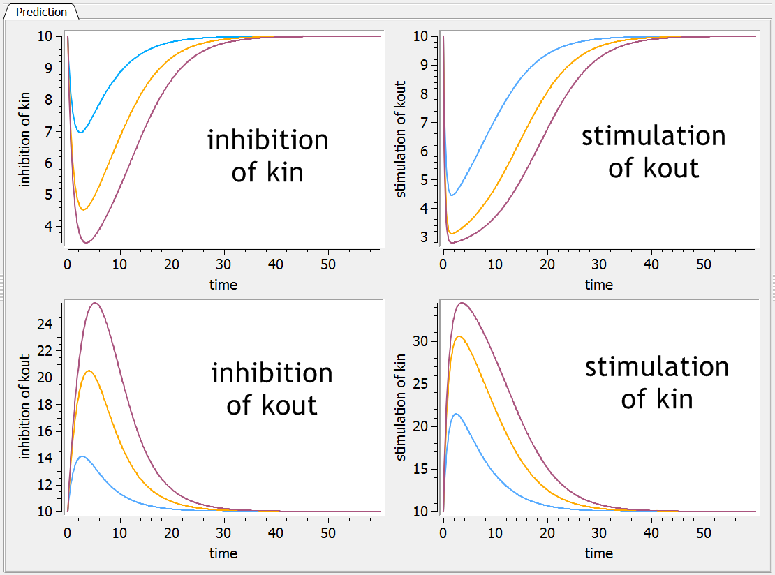
The 4 models have been implemented in an Mlxplore project for comparison. The Mlxplore script reads:

<MODEL>
[LONGITUDINAL]
input = {V, k, kin, kout, Imax1, IC501, gamma1, Imax2, IC502, gamma2, Emax3, EC503, gamma3, Emax4, EC504, gamma4}

EQUATION:
Cc=pkmodel(V,k)

odeType=stiff
t_0 = 0
R1_0 = kin/kout
R2_0 = kin/kout
R3_0 = kin/kout
R4_0 = kin/kout

ddt_R1 = kin*(1-Imax1* Cc^gamma1/(Cc^gamma1+IC501^gamma1)) - kout*R1
ddt_R2 = kin - kout*(1-Imax2* Cc^gamma2/(Cc^gamma2+IC502^gamma2))*R2
ddt_R3 = kin*(1+Emax3* Cc^gamma3/(Cc^gamma3+EC503^gamma3)) - kout*R3
ddt_R4 = kin - kout*(1+Emax4* Cc^gamma4/(Cc^gamma4+EC504^gamma4))*R4

<PARAMETER>
V = 10
k = 0.1
kin = 10
kout = 1
Imax1 = 0.8
IC501 = 10
gamma1 = 2
Imax2 = 0.8
IC502 = 10
gamma2 = 2
Emax3 = 3
EC503 = 10
gamma3 = 2
Emax4 = 3
EC504 = 10
gamma4 = 2

<DESIGN>
[ADMINISTRATION]
adm100 = {time=0, amount=100}
adm200 = {time=0, amount=200}
adm300 = {time=0, amount=300}

<OUTPUT>
list={R1,R2,R3,R4}
grid=0:0.1:60

<RESULTS>
[GRAPHICS]
p1 = {y={R1}, ylabel='inhibition of kin', xlabel='time'}
p2 = {y={R4}, ylabel='stimulation of kout', xlabel='time'}
p3 = {y={R2}, ylabel='inhibition of kout', xlabel='time'}
p4 = {y={R3}, ylabel='stimulation of kin', xlabel='time'}

The resulting dynamics of the response for 3 different doses for each model is depicted below: