Introduction
The function pkmodel permits to define common PK models in a very concise way. The purpose of this macro is to simplify the modeling of classical pharmacokinetics. The PK model is inferred from the provided set of named arguments. Most of the arguments are optional, and the pkmodel function enables several parametrizations, to select different models of absorption, elimination, etc. With the pkmodel function, the most common PK models are available. The concentration within the central compartment is the main output of the function. If an effect compartment is defined, its concentration defines the second output. The administration of the doses is always supposed to be of type 1, and the default absorption is the IV bolus one. The label of the central compartment is 1. The pkmodel function can also be used within the block EQUATION: or the block PK:.
We first give typical examples and then list all possible arguments.
Examples
Example 1: One compartment model with intravenous (bolus or infusion) administration
Cc = pkmodel(V, Cl)
This simple set of named arguments for pkmodel defines a PK model with one central compartment of label 1, with the default intravenous bolus administration for doses of administration type 1 and a linear elimination with the clearance parametrization in Cl. The volume of the central compartment is V. The concentration in the central compartment is the output Cc of the function.
If a column is tagged as infusion duration or as infusion rate in the data, this is recognized by the pkmodel macro and the doses of administration type 1 with a non-empty infusion rate or duration are administered as an infusion instead of a bolus.
Example 2: Two-compartment model with first order absorption with lag time
- With elimination rates: parameters Tlag, ka, V, k, k12, k21
Cc = pkmodel(Tlag, ka, V, k, k12, k21)
- With clearances: parameters Tlag, ka, V, Cl, Q, V2
Cc = pkmodel(Tlag, ka, V, k=Cl/V, k12=Q/V, k21=Q/V2)
Note that it is not possible to give Q and V2 as direct input parameters. Instead, we give the recognized keywords k12 and k21, and defined them using Q, V and V2.
Example 3: Three-compartment model with zero-order absorption
Cc = pkmodel(Tk0, V, k, k12, k21, k13, k31)
Tk0 represents the duration of the zero-order absorption. k12 and k21 are the rates to and from the first peripheral compartment and k13 and k31 are the rates to and from the second peripheral compartment.
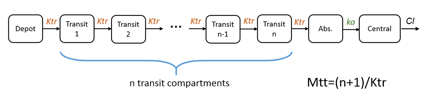
Example 4: One compartment model with transit compartments
Cc = pkmodel(ka, Mtt, Ktr, V, Cl)
In case of transit compartments, the mean transit time is defined as Mtt = (n+1)/Ktr with n the number of transit compartments (excluding the depot compartment and the absorption compartment) and Ktr the transit rate.
 The implementation is the same as described in Savic et al, “Implementation of a transit compartment model for describing drug absorption in pharmacokinetic studies” (2007), except that to approximate the factorial n!, we use the gamma function, which is more precise, instead of the Stirling formula.
Note that this model has no analytical solution, so the ODE system is used.
Example 5: One compartment model with effect compartment
{Cc, Ce} = pkmodel(ka, V, Cl, ke0)
The one-compartment model is connected to an effect compartment with a bi-directional rate ke0. The concentration in the effect compartment is called Ce in this example and can for instance be used to define a PD model.
Example 6: Model using almost all arguments
{Cc, Ce} = pkmodel(Tlag, ka, p, V, Vm, Km, k12, k21, k13, k31, ke0)
This more complex set of named arguments for pkmodel defines a PK model of one central compartment, with a first order absorption of rate ka for doses of administration type 1, and a Michaelis-Menten elimination of parameters Vm and Km. The volume of the central compartment is V. The concentration in the central compartment is the first output Cc of the function. An effect compartment is defined with a rate ke0 and its concentration is the second output Ce. Two peripheral compartments of labels 2 and 3 are linked to the central compartment of label 1. The respective couples of exchange rates are (k12, k21) and (k13, k31). The first order absorption has a lag time Tlag and the absorbed amount is scaled with a proportion of p.
List of arguments
The complete set of named arguments and output for pkmodel follows. They belong to the central compartment, the absorption process, the elimination process, the exchanges with the peripheral compartments, or an effect compartment. Some arguments are mutually exclusive, or require other ones to be also defined. Most of them are optional, so the mandatory arguments are stated.
Arguments for the central compartment
-
- Cc = pkmodel(…): The first output is the concentration within the central compartment. Another name can be used. Mandatory.
- V: Volume of the central compartment. Mandatory.
Arguments for the absorption process of a standard PK model
-
- Tk0: Defines a zero order absorption of duration Tk0. Excludes ka, Ktr and Mtt.
- ka: Defines a first order absorption of rate ka. Excludes Tk0.
- Ktr: Along with ka and Mtt, defines an absorption with transit compartments, with transit rate Ktr. Excludes Tk0.
- Mtt: Along with ka and Ktr, defines an absorption with transit compartments, with mean transit time Mtt. Excludes Tk0.
- Tlag: Lag time before the absorption.
- p: Final proportion of the absorbed amount. Can affect the effective rate of the absorption, not its duration.
- default if no argument supplied for the absorption process: iv bolus
Arguments for the elimination process of a standard PK model
-
- k: Defines a linear elimination of rate k. Excludes Cl, Vm and Km.
- Cl: Along with V, defines a linear elimination of clearance Cl. Excludes k, Vm and Km.
- Vm: Along with V and Km, defines a Michaelis-Menten elimination of maximum elimination rate Vm. Units of Vm are amount/time. Excludes k and Cl.
- Km: Along with V and Vm, defines a Michaelis-Menten elimination of Michaelis-Menten constant Km. Units of Km are concentration so amount/volume. Excludes k and Cl.
Arguments for the peripheral compartments of a standard PK model
-
- k12: Along with k21, defines a peripheral compartment 2 of input rate k12.
- k21: Along with k12, defines a peripheral compartment 2 of output rate k21.
- k13: Along with k31, defines a peripheral compartment 3 of input rate k13.
- k31: Along with k13, defines a peripheral compartment 3 of output rate k31.
Arguments for the effect compartment of a standard PK model
-
- {Cc, Ce} = pkmodel(…): The second output is the concentration within the effect compartment. Another name can be used.
- ke0: Defines an effect compartment with transfer rate ke0 from the central compartment.
Additional possibilities
Knowing the label of the central compartment (cmt=1) and the administration type supported by the function pkmodel (type=1), one can build up a custom PK model by adding other PK elements to a base standard PK model. Referencing this label and administration type of value 1 allows to connect the additional PK elements.
Overview of arguments
Overview of input arguments for the pkmodel() macro
Rules
- Only one type of administration is allowed
- Only one pkmodel function is allowed in the Mlxtran file
- Arguments must be from the list of defined arguments for pkmodel. Arguments with different names are not recognised.
- pkmodel can not be used together with any macros for the administration. The administration is defined exclusively with the arguments supplied to pkmodel()
- A pkmodel output can be used with ODEs or with macros.
- pkmodel can also be defined in the PK: block or the EQUATION: block.