This page presents the count model library proposed by Lixoft from the 2019 version on. It includes a short introduction on count data, the different ways to model this kind of data, and typical models.
- What is count data
- Formatting of count data in the MonolixSuite
- Important concepts: the probability mass function
- Encoding of count models in the MonolixSuite
- Library of parametric models for count data
- Case studies
What is count data
Count data come from counting something, e.g., the number of trials required for completing a given task. The task can for instance be repeated several times (longitudinal count data) and the individuals performance followed.
Count data can also represent the number of events happening in regularly spaced intervals, e.g the number of seizures every week. If the time intervals are not regular, the data may be considered as repeated time-to-event interval censored, or the interval length can be given as regressor to be used to define the probability distribution in the model.
Formatting of count data in the MonolixSuite
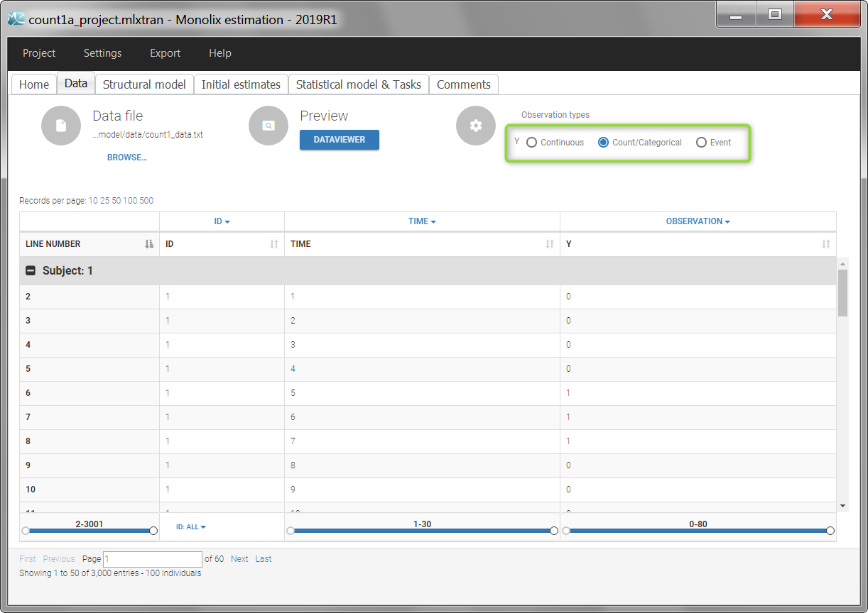
Count data can take only non-negative integer values. The counts for each individual are recorded in the OBSERVATION column-type. If the data is longitudinal (over time), the times at which the counts have been recorded are indicated in the TIME column-type. If the data is not longitudinal, the TIME column is still necessary and a time of 0 can be used for instance.
ID TIME Y
1   0   8
1   4   9
1   8   11
2   0   6
2   4   6
2   8   7
In the example above, the values in the time column can either indicate the time at which the counts have been counted, or the start or end time of the period over which the number of events are recorded.
In the Monolix GUI, the user must indicate that the data is of type Count/Categorical:
Important concept: the probability mass function
Count data are described by their probability mass function, which gives the probability that the discrete random variable is exactly equal to some value: \( \mathbb{P}(y_{ij}=k) \) with \(y_{ij}\) the observed count number for individual \(i\) at time \(j\) and \(k>0\).
For instance the probability mass function for a Poisson distribution is:
\(\mathbb{P}(y_{ij}=k)=\frac{\lambda^k e^{-\lambda}}{k!} \)
If \(\lambda=3\), then the probability of having a count of 0 is 4.9%, a count of 1 is 14.9%, a count of 2 is 22.4%, a count of 3 is 22.4%, etc.
Encoding of count models with the MonolixSuite
In Monolix, a model for count data is defined via the probability mass function, which in a population approach typically depends on individual parameters: \( \mathbb{P}(y_{ij}=k) = f(t_j,\psi_i)\).
The typical syntax to define the random variable representing the count number is the following:
DEFINITION:
CountNumber = {type=count, P(CountNumber=k) = ...}
CountNumber is the name of the random variable and can be replaced by another name. On the opposite, k is a mandatory name for the values. The random variable CountNumber is then listed in the outputs, to be matched to the observed data.
The probability mass functions often involve ratios of factorials. While the ratio is often a reasonable value, the numerator and denominator can be huge values that are difficult to handle numerically. It is therefore better to work with the log of the factorials. The function for log factorial in Mlxtran language is factln() (for integers). To extend the factorials to the continuous domain, the gamma function can be useful: \( \Gamma(n)=(n-1)!\). The log of the gamma function corresponds to the gammaln() function in Mlxtran. It is possible to define directly the log of the probability mass function with:
DEFINITION:
CountNumber = {type=count, log(P(CountNumber=k)) = ...}
For instance to define a binomial distribution, we can write:
DEFINITION:
Y = {type=count, log(P(Y=k)) = gammaln(n+1) - factln(k) - gammaln(n-k+1) + k*log(p) + (n-k)*log(1-p)}
where gammaln() is used for terms that can be non-integers and factln() for terms that are integers.
It is possible to use “if” statements related to \(k\) in the definition of the probability mass function by using the syntax below. This can be useful to define zero-inflated models for instance. The “if” statements relating to time, regressors, or parameters values can be put in a EQUATION: section before the DEFINITION: block.
DEFINITION:
CountNumber = {type=count,
if k==0
Pk = ...
else
Pk = ...
end
P(CountNumber=k) = Pk}
The parameters involved in the definition of the probability mass function (for instance \(\lambda\) for a Poisson distribution) can be identical for all individuals, or vary from individual to individual. This is defined in the section “Individual model” of the graphical interface as usual. These parameters can also evolve over time or be a function of other variables such as drug concentration or tumor burden for instance. See the demo “PKcount_project.mlxtran” for instance in the Monolix demo folder, section 4.2.
Library of models for count data
To describe the various shapes that a count distribution can take, we have developed a library of models. The library includes the most typical distributions, their zero-inflated counterpart, and several options for the evolution of time of the main parameter:
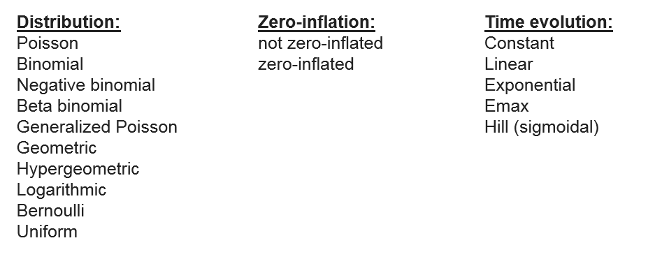
The probability mass functions and a description of the parameters is given below:

Case studies
[coming soon]