1.Mlxtran, a human readable language for model description
Mlxtran
Model typesThe mlxtran language can be used to describe a wide variety of models, including models for continuous, count, categorical and time-to-event data. The main output of an |
|
Mlxtran model structure
Mlxtran can be used to represent models for parameter estimation with Monolix or for simulation with Simulx. In Monolix, the model file (with .txt extension) contains only the structural part of the model (section [LONGITUDINAL]), while the statistical part of the model (covariate effects, parameter distributions and error model) is defined through the graphical user interface. When saving a Monolix project, the statistical part of the model is written in the .mlxtran project file using mlxtran language.
In Simulx, the model file contains the [LONGITUDINAL] section, but can also contain the [COVARIATE] and [INDIVIDUAL] sections to describe the statistical part of the model. When a Monolix project is imported into Simulx, the model with all sections is created automatically from the .txt monolix model file and .mlxtran monolix project file. When starting a Simulx project from scratch, the [LONGITUDINAL] section is mandatory and the [COVARIATE] and [INDIVIDUAL] sections are necessary if covariates and inter-individual variability are present in the model.
- [LONGITUDINAL]: structural model and error model
- [INDIVIDUAL]: parameter distributions
- [COVARIATE]: covariate declaration and transformations
- [POPULATION]: only compatible for simulations with mlxR, in combination with MonolixSuite 2019 and before.
The sections are themselves divided into blocks, which allow to define different types of variables in different ways:
- DESCRIPTION: block to put comments on the model
- PK: block were macros can be used to define compartments and transfers between them
- EQUATION: block were ODEs can be defined, as well as mathematical expressions (e.g parameter transformations)
- DEFINITION: block to define random variables (discrete or continuous) via their probability distribution
- within the [LONGITUDINAL] section: error model, probability distribution for count/categorical output and hazard for time-to-event output
- within the [INDIVIDUAL] section: distribution of the parameters
- OUTPUT: block indicating the output of the model
Below we show the possible sections and blocks for Monolix and Simulx.

2.[LONGITUDINAL]
Description
The [LONGITUDINAL] section is used to describe the structural model and the observation model discrete and time-to-event data. In Simulx it is also used to define the error model for continuous observations.
Scope
The [LONGITUDINAL] section is mandatory for all Mlxtran models for Monolix and Simulx.
Inputs
In Monolix, the input = { } list of the [LONGITUDINAL] section declares the individual parameters and the regressors. In Simulx, the error model parameters also also declared in the input (while this is done automatically via the GUI in Monolix). The inputs can have been defined in the [INDIVIDUAL] section, or be global variables defined via the Monolix or Simulx GUI.
For regressors, the regressor status must be specified using the following syntax, for instance for a regressor called regvar. One line per regressor is necessary. As a reminder, in Monolix, the regressors are mapped to the regressor columns of the data set by declaration order (first column tagged as regressor mapped to the first regressor appearing in the input list).
regvar = {use=regressor}
The inputs of [LONGITUDINAL] specified as regressors will be recognized as such and appear in the regressor element in Simulx GUI. Inputs of [LONGITUDINAL] which have been defined in the DEFINITION block of the [INDIVIDUAL] section will be recognized as individual parameters. All others (in particular error model parameters) will be recognized as population parameters in Simulx.
Example for Monolix:
In this example, ka, V, Cl, Emax and EC50 are individual parameters and E0 is declared as a regressor and will be read from the first data set column tagged as regressor.
[LONGITUDINAL]
input = {ka, V, Cl, E0, Emax, EC50}
E0 = {use = regressor}
Example for Simulx:
In this example, in addition to the individual parameters ka, V, Cl, Emax and EC50 and the regressor E0, population error model parameters a and b are also defined.
[LONGITUDINAL]
input = {ka, V, Cl, E0, Emax, EC50, a, b}
E0 = {use = regressor}
Outputs
In Monolix, the OUTPUT: block declare the variables which will be mapped to the observations in the data set via the output={} list, and the additional variables recorded in the output tables via the table={} list. The outputs are mapped to the observation ids of the data set via the mapping panel in the Monolix GUI. The variables in the table={} statement are outputted in the result folder of Monolix.
In Simulx, variables listed in table={} or output={} will have an output element generated automatically. It is also possible to request any model variable as output in Simulx, no matter if it has been declared in the OUTPUT section or not.
Note that from the 2020R1 version, the OUTPUT: section is mandatory.
Example:
OUTPUT:
output = {Conc, Effect}
table  = {Ap, T12}
Usage
The [LONGITUDINAL] section can contain three different blocks. The PK: block permits to define PK models using macros, and to link the administration information of the data set with the model. The EQUATION: block is for mathematical equations including ODEs and DDEs. The DEFINITION: block is used to define a random variable and its probability distribution.
In all blocks, it is possible to use:
- if/else statements with logical operators
- mathematical functions
- keywords for the time and dose-related events
- regressors
Reserved keywords of the Mlxtran language cannot be used as names for other parameters. Mlxtran is a declarative language, not an imperative language. Therefore equations are mathematical definitions rather than a series of instructions.
PK: block
In the PK: block, macros can be used to define compartmental models using base building blocks.
- pkmodel() macro: allows to define typical PK models in one line
- compartment(), peripheral(), effect(), transfer(), depot(), oral(), iv(), elimination(), empty() and reset() macros: allow to build models part by part
EQUATION: block
In the EQUATION: block, ODEs and DDEs can be defined.
DEFINITION: block
The DEFINITION: block is used to define random variable, which represent observations. The observations can be continuous, count, categorical or time-to-event. In Monolix, only count, categorical and time-to-event observation models are defined in the structural model file, while the continuous error models are defined in the GUI. In Simulx, they are all defined in the model file.
Library of models and examples
The MonolixSuite contains libraries of pre-written structural models which can be directly selected via the GUI in Monolix or Simulx:
- PK: typical pharmacokinetics models with several types of administrations and 1 to 3 compartments
- PK/PD: joint PK/PD model with direct effect, effect compartment or turnover
- PK double absorption
- TMDD: target mediated drug disposition models
- TTE: time-to-event models
- Count: models for count data
- TGI: tumor growth and tumor growth inhibition models
For common models which are not (yet) in the libraries, we provide an example page.
2.1.Input definition
The [LONGITUDINAL] section starts with the declaration of its inputs. These parameters can come from:
- the calling software: Monolix, Simulx or Mlxplore
- the outputs of the section [INDIVIDUAL],
- the parameters defined in the section <PARAMETER> .
For Monolix all parameters in the input = { } list define the parameters that are estimated or used as regressor variables. Notice that outputs from the [COVARIATE] section can not be used as inputs for the [LONGITUDINAL] section.
For example, for a model where a function f depends on a vector of input parameters ")
 = \frac{D, k_a}{V(k_{a} - k)}(e^{-kt} - e^{-k_{a}t})")
The input is defined in the following
DESCRIPTION: Model description with an analytical expression
[LONGITUDINAL]
input = {ka, V, k}

EQUATION:
D = 100
f = D*ka/(V*(ka-k))*(exp(-k*t) - exp(-ka*t))
Notice that, in this example, the parameter D is a fixed constant of the model and is thus not defined as an input.
2.2.Modelling ODEs
Introduction
Ordinary differential equations (ODEs) can be implemented in the EQUATION: block of the [LONGITUDINAL] section. The ODEs describe a dynamical system and are defined by a set of equations for the derivative of each variable, the initial conditions, the starting time and the parameters.
Derivatives
The keyword ddt_ in front of a variable name, as ddt_x and ddt_y, defines the derivative of the ODE system with respect to time. The variable names denote the components of the solution. These variables are defined at the whole [LONGITUDINAL] section level through their derivatives. The derivatives themselves aren’t variables but keywords, and cannot be referenced by other equations nor be defined under a conditional statement.
Initial conditions
The keyword t_0 defines the initial time of the differential equation, while the variable names with suffix _0 define the initial conditions of the system. More precisely, in a differential equation for the variable x, x is defined at t = t0 by the initial condition x_0, i.e. x(t0)=x_0 and by the differential equation after t0.
Linking administration with ODEs
Mlxtran provides the PK macro depot() that can be used to link the administration from a data set with the model. Details and examples how to use depot() for the administration are given here.
Example
We consider in this example a first order differential equation on x defined by:
=V,~~\textrm{for}~~t\leq10\end{array}\right.")
where (V,k)=(10,.05), this ODE is typically a linear elimination process of a volume. This model is implemented in the file mlxt_ode.txt:
DESCRIPTION: Model description with a simple ODE representing a linear elimination precess of a volume
[LONGITUDINAL]
input = {V, k}

EQUATION:
t_0 = 10
x_0 = V
ddt_x = -k*x
Stiff ODEs
A numerical algorithm providing an efficient and stable way to solve the ODEs and DDEs is used to compute the solution of the dynamical models. Different numerical algorithms can be used to solve the ODE depending on the properties of the ODE system (Adams methods for non stiff ODEs, and Backward Differentiation Formulas methods for stiff ODEs). The right numerical algorithm must be selected in order to get an accurate and stable solution within a reasonable computational time. The stiffness of an ODE systems is one of the main properties that influences the choice of the numerical algorithms. Stiff ODEs can lead to very long computational times if an inappropriate algorithm is used. Stiff ODEs are typical for models that include processes taking place at different time scales. For example models with reaction and diffusion processes are known to be stiff. Reactions can occur at the seconds time scale while diffusion processes can take hours. For such cases a dedicated numerical algorithm for stiff ODEs is available.
A solver for stiff ODEs can be selected in Mlxtran using the keyword odeType. There are two possible choices for odeType:
; ode is considered as stiff
odeType = stiff
; ode is considered as non-stiff (default)
odeType = nonStiff
This command has to be defined in the [LONGITUDINAL] section. When odeType is not specified then the nonStiff ODE solver is used by default.
Note that:
- For the DDEs, the keyword odeType is ineffective.
- For many ODEs the nonStiff solver will provide the best solution. However, it is good practice to always test both solvers to see which one is providing the shorter computational time.
ODE solver tolerances
The stiff and non-stiff solvers compute the solution of the ODE system up to a certain precision, which is defined through the tolerance. The values by default are the following:
- non-stiff solver: absolute tolerance 1e-6, relative tolerance 1e-3
- stiff solver: absolute tolerance 1e-9, relative tolerance 1e-6
The tolerances can be modified by specifying the desired value in the structural model file using the keywords odeAbsTol and odeRelTol, for instance:
EQUATION:
odeAbsTol = 1e-12
odeRelTol = 1e-9
The smaller the tolerance, the closer the computed prediction will be from the true solution. The absolute tolerance indicates how much the absolute difference between the computed prediction \(y_{solver}\) and the true solution \(y_{true}\) can be, i.e \(|y_{solver}-y_{true}|<\textrm{odeAbsTol}\). The relative tolerance is related to the number of digits which are correct, i.e \(\frac{|y_{solver}-y_{true}|}{|y_{true}|}<\textrm{odeRelTol}\).
Note that the right hand side needs to be a number (such as odeAbsTol=1e-12 or odeAbsTol=0.000001) and cannot be an expression (odeAbsTol=10^(-9) is not accepted).
Rules and Best Practices
- We encourage the users to define the initial conditions explicitly, although the default initial value is x_0=0.
- When no starting time t0 is defined in the Mlxtran model for Monolix then by default t0 is selected to be equal to the first dose or the first observation, whatever comes first.
- If t0 is defined, a differential equation needs to be defined.
- Initial conditions can depend on
- time
- an input parameter. Therefore, initial condition values can also be estimated in Monolix.
- a regressor value. In that case, again, a differential equation needs to be defined.
- Only first order differential equation can be used with Mlxtran. If you want to use a differential equation of the form
, you need to transform the higher order differential equation into a first order differential equations by defining n successive differential equations as proposed in the following “Best Practices Ex. 1: Second order differential equation”.
- The derivatives of a ODE system cannot be conditional, i.e. ddt_ cannot be used within an if statement. Instead, conditional intermediate variables for the values of the derivatives should be used as shown in “Best Practices Ex. 2: IF statement”. A conditional statement can be built by combining the keywords if, elseif, else and end. Several elseif keywords can be chained, and the conditions are exclusive in sequence. A default value can be provided using the keyword else, but also as a simple definition preceding the conditional structure. An unspecified conditional value is null. The enclosed variables are not local variables, which means that a variable with remaining conditional definitions is still incomplete and cannot be referenced into another definition, even under the same condition.
") , you need to transform the higher order differential equation into a first order differential equations by defining n successive differential equations as proposed in the following “Best Practices Ex. 1: Second order differential equation”.
, you need to transform the higher order differential equation into a first order differential equations by defining n successive differential equations as proposed in the following “Best Practices Ex. 1: Second order differential equation”.Best Practices Ex. 1: Second order differential equation
If you want to use a second order differential equation of the type 
,\dot{x}(0))=(a,b)")
Mlxtran writes
[LONGITUDINAL]
input = {a, b}

EQUATION:
t0 = 0
x_0 = a
dx_0 = b
ddt_x = dx
ddt_dx = -x-dx
Best Practices Ex. 2: IF statement
If a parameter value depends on a condition, it can be written with in Mlxtran with the usual if-else-end syntax. For example, if a parameter c should be 1 if t<=10, 2 if t<20 and 3 otherwise, write
if t<=10
   c = 1
elseif t<20
   c = 2
else
   c = 3
end
Derivatives cannot be written within an if-else-end structure. Instead, intermediate variables should be used. For example, if a derivative of x over time should be 1 if t<=10 and 2 otherwise, write
if t<=10
   dx = 1
else
   dx = 2
end
ddt_x = dx
2.3.Delayed differential equations (DDE)
Introduction
Delayed differential equations (DDEs) can be implemented in a block EQUATION: of the section [LONGITUDINAL]. For that, the function delay is proposed. This function allows to delay a dynamical variable by a constant time. One can also build a model with several delays. Delays in the absorption after drug administration must be implemented using the keyword Tlag in the administration macros.
Since the DDE solver is slower than the ODE solver, we recommend the alternative implementation using ODEs only and presented in the following video, when possible, as it leads to greatly shorter run times.
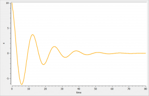
Example
We consider in this example a first order delay differential equation on x defined by:
 = k_ax(t)-kx(t-\tau)")
This DDE is typically an accumulation process with a delayed linear elimination treatment. This model is implemented in the file mlxt_dde.txt:
DESCRIPTION: Model description with a delay
[LONGITUDINAL]
input = {V, ka, k, tau}

EQUATION:
t0 = 0
x_0 = V
ddt_x = ka*x-k*delay(x,tau)
The result of the simulation is performed by Mlxplore using (V=10, k=0.5, k=.25, tau=2) and is proposed on the following figure. The interesting part in this example is that the delay has an important impact on the stability of the system. This kind of systems can thus be explored by Mlxplore.
Rules
- The delay function can delay a “pure” component in a dynamical equation. There are three main things to point out and we will discuss the three of them:
- By pure, we mean that the function can not take state calculations into account. In the previous example, if we had used delay(k*x,tau) instead of k*delay(x,tau), this would have generated an error.
- By component, we mean that the delay function can only delay variable with a dynamic behavior (defined by a derivative equation). In the previous example,using the delay function with anything else than x would lead to an error.
- By dynamical equation, we mean that the delay function should be called directly in a ddt_ equation. For example, if we have in addition a DDE of the form
, one could be tempted to implement it in
Mlxtranunder the following incorrect form:z = delay(x,1) ddt_y = z-y
It should be defined directly as
ddt_y = delay(x,1)-y
The first implementation would lead to an error.
- The delay must remain constant over the time.
- It is good practice to define the initial conditions of the DDE system (t0 and initial values for the variables). If the initial condition is not defined, then it is set to the default value 0. Notice that you can have varying initial conditions. Note also that an initialization can be performed if the values can be analytically computed. For example, we can define
, and it would be translated in
Mlxtranunder the formx_0 = V*(1+t)
=x(t-1)-y(t)") , one could be tempted to implement it in
, one could be tempted to implement it in ![x(t)=V(1+t)~~\forall t\in[-1,0]](http://s0.wp.com/latex.php?latex=x%28t%29%3DV%281%2Bt%29%7E%7E%5Cforall+t%5Cin%5B-1%2C0%5D&bg=ffffff&fg=000&s=0 "x(t)=V(1+t)~~\forall t\in[-1,0]") , and it would be translated in
, and it would be translated in 2.4.Regression variables
A regression variable is a variable x that depends on time but is not defined in the model but rather is defined in the data set in the case of Monolix. In the data set the regression variable is represented by vector ")
")
")

Note that x is only defined at time points
=x_j~~\text{for}~~t_j \leq t < t_{j+1}")
Regression variables are used in the Mlxtran model by defining them as a list in the regressor block of the [LONGITUDINAL] section:
[LONGITUDINAL]
input = {reg_var1, reg_var2, ....}
reg_var1 = {use = regressor}
reg_var2 = {use = regressor}
...
For each regression variable defined in the regressor list of the Monolix Mlxtran model, there must be a column in the data set defined as a regressor column X. Regressors in the data set and in the Monolix Mlxtran model are matched by order, not by name.
2.5.Observation models for continuous data
Purpose
The observation model is the link between the prediction f of the structural model and the observation. Thus, the observational model is an error model representing the noise and the uncertainty of the measurements. The observation model can be defined only in the Monolix interface or the Mlxtran file in Simulx.
Possible observation models
For the continuous observations, the general form u(y) = u(f) + g e is considered where e is a sequence of independent random variables normally distributed with mean 0 and variance 1, and u is the transformation associated with the distribution of the observations. It is also possible to assume that the residual errors are correlated. Following is a list of distributions and residual error models that can be selected in the Monolix user interface.
Residual error models
- constant: constant error model
- proportional: proportional error model + power
- combined1: combined error model + power
- combined2: combined error model + power
(equivalent to
where e1 and e2 are sequences of independent random variables normally distributed with mean 0 and variance 1)


e")
^2}e") (equivalent to
(equivalent to  where e1 and e2 are sequences of independent random variables normally distributed with mean 0 and variance 1)
Notice that the parameter c is fixed to 1 by default. However, it can be unfixed and estimated.
Positive gain on the error model
The second parameter b in the observational models comb1 and comb1c can be forced to be always positive by selecting b>0.
Distributions
- normal: u(y) = y. This is equivalent to no transformation.
- lognormal: u(y) = log(y). Thus, for a combined error model for example, the corresponding observation model writes \(\log(y) = \log(f) + (a + b\log(f)) \varepsilon\). It assumes that all observations are strictly positive. Otherwise, an error message is thrown. In case of censored data with a limit, the limit has to be strictly positive too.
- logitnormal: u(y) = log(y/(1-y)). Thus, for a combined error model for example, corresponding observation model writes \(\log(y/(1-y)) = \log(f/(1-f)) + (a + b\log(f/(1-f)))\varepsilon\). It assumes that all observations are strictly between 0 and 1. However, we can modify these bounds to define the logit function between a minimum and a maximum, and the function u becomes u(y) = log((y-y_min)/(y_max-y)). Again, in case of censored data with a limit, the limits has to be strictly in the proposed interval too.
Hence, the following observation models can be defined with a combination of distribution and residual error model:
- exponential error model:
and
→ constant error model and a lognormal distribution
- logit error model
→ constant error model and a logitnormal distribution
- band(0,10):
→ constant error model and a logitnormal distribution with min and max at 0 and 10 respectively
- band(0,100):
→ constant error model and a logitnormal distribution with min and max at 0 and 10 respectively
 = \log(y)") and
and  = \log(\frac{y}{1-y})")
 = \log(\frac{y}{10-y})")
 = \log(\frac{y}{100-y})")
Mlxtran observational model syntax
The DEFINITION: block in the [LONGITUDINAL] section is used to define the observational model:
DEFINITION:
observationName = {distribution = distributionType, prediction = predictionName, errorModel = errorModel(param)}
(notice that one can use type=continuous instead of distribution = distributionType)
For example, if the observation is a concentration with a combined error model (Concentration = Cc + (a+b*Cc)*e), the observational error model is written as
DEFINITION:
Concentration= {distribution = normal, prediction = Cc, errorModel=combined1(a, b)}
When the observational error is defined in the Mlxtran model file, the user must declare the observational model parameters (a and b in the presented example) as inputs.
Rules and best practices
- The eventual arguments of the error model can not be calculations, only input names.
- In Monolix, the user can choose the error model through the interface.
- In Monolix, the name of the error models input parameters can not have any name.
- The name of the input should correspond to the definition of the error model (ex. a for a constant error model, b for a proportional error model, (a,b) for a combined1 error model, …)
- If there are several continuous outputs, the names of the error models input parameters should be linked to the order of the outputs (1 for the first error model, …)
- For example, for a single output, a combined error model writes without any number as follows
DEFINITION: Concentration = {distribution = normal, prediction = Cc, errorModel=combined1(a, b)} - For example, for two outputs, a combined error model and a constant error model write as follows
DEFINITION:
Concentration = {distribution = normal, prediction = Cc, errorModel=combined1(a1, b1)}
PCA = {distribution = normal, prediction = E, errorModel=constant(a2)}
- Notice that a parameter can not be shared by two error models. For example, in the previous Concentration/PCA example, we can not replace a2 by a1.
2.6.Observation model for count data
Use of count data
Longitudinal count data is a special type of longitudinal data that can take only nonnegative integer values {0, 1, 2, …} that come from counting something, e.g., the number of seizures, hemorrhages or lesions in each given time period. In this context, data from individual i is the sequence \(y_i=(y_{ij},1\leq j \leq n_i)\) where \(y_{ij}\) is the number of events observed in the jth time interval \(I_{ij}\).
Count data models can also be used for modeling other types of data such as the number of trials required for completing a given task or the number of successes (or failures) during some exercise. Here, \(y_{ij}\) is either the number of trials or successes (or failures) for subject i at time \(t_{ij}\). For any of these data types we will then model \(y_i=(y_{ij},1\leq j \leq n_i)\) as a sequence of random variables that take their values in {0, 1, 2, …}. If we assume that they are independent, then the model is completely defined by the probability mass functions \(\mathbb{P}(y_{ij}=k)\) for \(k \geq 0\) and \(1 \leq j \leq n_i\). Here, we will consider only parametric distributions for count data.
Observation model syntax
Considering the observations as a sequence of conditionally independent random variables, the model is completely defined by the probability mass functions \(P(y_{ij}=k)\). An observation variable for count data, with name Y for instance, is defined using the following syntax:
DEFINITION:
Y = {type=count, P(Y=k) = ...}
- type=count: indicates the data type
- P(Y=k): probability of a given count value
k, for the observation namedY. The observation name is free but must be the same at the beginning of the line and for the probability definition.kis a reserved keyword and represents a positive integer. k supersedes in this scope any variable k defined previously. The probability must be in [0,1].
A transformed probability can also be provided. The transformation can be log, logit, or probit. For instance with a log-transformation:
DEFINITION:
Y = {type=count, log(P(Y=k)) = ...}
As k is only recognized within the probability definition, it is not possible to define the probability using k in an EQUATION block above. However, it is possible to use if/else statements within the probability definition:
DEFINITION:
Y = {type=count,
if k==0
Pk = ...
else
Pk = ...
end
P(Y=k) = Pk}
Common mathematical functions to define count distributions are factorial(a), factln(a) (logarithm of factorial) and gammaln(a) (logarithm of gamma function). They can be used with a any positive numerical value (not only integers). Note that factorials grow very rapidly and can be considered as “+infinity” in a computer, even when the probability is defined as a ratio of two factorials which stays with reasonable values on paper. It is thus convenient to works with logarithms of factorials, which grow much slower (see examples).
Examples
Example 1: Poisson distribution with time evolution
In this example, the Poisson distribution is used for defining the distribution of \(y_j\):
$$y_j \sim \textrm{Poisson}(\lambda_j) \iff P(Y=k)=\frac{\lambda_j^k e^{-\lambda_j}}{k!}$$
where the Poisson intensity \(\lambda_j\) is function of time \(\lambda_j = a+bt_j\). This model is implemented as follows
[LONGITUDINAL]
input = {a,b}

EQUATION:
lambda = a+b*t

DEFINITION:
y = {type=count, P(y=k) = exp(-lambda)*(lambda^k)/factorial(k)}
Example 2: Binomial distribution
We consider n Bernouilli trials, each having a probability of success p. The probability of having k successes is:
$$P(Y=k)=\frac{n!}{k!(n-k)!}p^k(1-p)^{n-k}$$
To avoid that \(k!\) be so large that it will be considered as NaN by a computer, it is good practice to define the log of the probability to convert the ratios of large number into a sum of smaller numbers:
$$\log(P(Y=k))=\log(n!) – \log(k!) – \log((n-k)!) + k \log(p) + (n-k) \log(1-p)$$
The corresponding Mlxtran model is:
[LONGITUDINAL]
input = {n, p}

DEFINITION:
CountNumber = {type=count, log(P(CountNumber=k)) = gammaln(n+1) - factln(k) - gammaln(n-k+1) + k*log(p) + (n-k)*log(1-p)}

OUTPUT:
output = Y
Example 3: Poisson distribution with zero inflation
Zero-inflations can be encoded using if/else statements:
[LONGITUDINAL]
input = {lambda, f}

DEFINITION:
CountNumber = {type=count,
if k==0
Pk = exp(-lambda)*(1-f) + f
else
Pk = exp(k*log(lambda) - lambda - factln(k))*(1-f)
end
P(CountNumber=k) = Pk}

OUTPUT:
output = CountNumber
Library of count models
The MonolixSuite library of models includes many pre-written count data models: Count library.
2.7.Observation model for categorical data
- Observation model for categorical ordinal data
- Observation model for categorical data modeled as a discrete Markov chain
- Observation model for categorical data modeled as a continuous Markov chain
Observation model for categorical ordinal data
Use of categorical data
Assume now that the observed data takes its values in a fixed and finite set of nominal categories 
")
")


![\mathbb{P}(y_{ij}=c_k | \psi_i) \in [0,1]](http://s0.wp.com/latex.php?latex=%5Cmathbb%7BP%7D%28y_%7Bij%7D%3Dc_k+%7C+%5Cpsi_i%29+%5Cin+%5B0%2C1%5D&bg=ffffff&fg=000&s=0 "\mathbb{P}(y_{ij}=c_k | \psi_i) \in [0,1]")
 =1")


We can think, for instance, of levels of pain (low ")

")

 \leq \mathbb{P}(y_{ij} \preceq c_2 | \psi_i)\leq \ldots \leq \mathbb{P}(y_{ij} \preceq c_K | \psi_i) =1 .")
It is possible to introduce dependence between observations from the same individual by assuming that ")


 = \mathbb{P}(y_{ij} = c_k | y_{i,j-1},\psi_i).")
Observation model syntax
Considering the observations as a sequence of conditionally independent random variables, the model is again completely defined by the probability mass functions
")

")
)")
- categories: List of the available ordered categories. They are represented by increasing successive integers.
- P(Y=i): Probability of a given category integer i, for the observation named Y. A transformed probability can be provided instead of a direct one. The transformation can be log, logit, or probit. The probabilities are defined following the order of their categories. They can be provided for events where the category is a boundary, instead of an exact match. All boundaries must be of the same kind. Such an event is denoted by using a comparison operator. When the value of a probability can be deduced from others, its definition can be spared.
Example
In the proposed example, we use 4 categories and the model is implemented as follows
[LONGITUDINAL]
input =  {th1, th2, th3}

DEFINITION:
level = {type = categorical, categories = {0, 1, 2, 3},
logit(P(level <=0)) = th1
logit(P(level <=1)) = th1 + th2
logit(P(level <=2)) = th1 + th2 + th3}
Using that definition, the distribution associated to the parameters are
- Normal for th1. Elsewise, it implies that logit(P(level <=0))>0 and thus that P(level <=0).
- Lognormal for th2 and th3 to make sure that P(level <=1)>P(level <=0) and P(level <=2)>=P(level <=1) respectively.
Observation model for categorical data modeled as a discrete Markov chain
Use of categorical data modeled as a Markov chain
In the previous categorical model, the observations were considered as independent for individual i. It is however possible to introduce dependence between observations from the same individual assuming that _{j=1,.., n_i}")
Observation model syntax
An observation variable for ordered categorical data modeled as a discrete Markov chain is defined using the type categorical, along with the dependence definition Markov. Its additional fields are:
- categories: List of the available ordered categories. They are represented by increasing successive integers. It is defined right after type.
- P(Y_1=i): Initial probability of a given category integer i, for the observation named Y. This probability belongs to the first observed value. A transformed probability can be provided instead of a direct one. The transformation can be log, logit, or probit. The probabilities are defined following the order of their categories. They can be provided for events where the category is a boundary, instead of an exact match. All boundaries must be of the same kind. Such an event is denoted by using a comparison operator. When the value of a probability can be deduced from others, its definition can be spared. The initial probabilities are optional as a whole, and the default initial law is uniform.
- P(Y=j|Y_p=i): Probability of transition to a given category integer j from a previous category i, for the observation named Y. A transformed probability can be provided instead of a direct one. The transformation can be log, logit, or probit. The probabilities are grouped by law of transition for each previous category i. Each law of transition provides the various transition probabilities of reaching j. They can be provided for events where the reached category j is a boundary, instead of an exact match. All boundaries must be of the same kind for a given law. Such an event is denoted by using a comparison operator. When the value of a transition probability can be deduced from others within its law, its definition can be spared.
Example
An example where we define an observation model for this case is proposed here
[LONGITUDINAL]
input = {a1, a2, a11, a12, a21, a22, a31, a32}

DEFINITION:
State = {type = categorical, categories = {1,2,3}, dependence = Markov
P(State_1=1) = a1
P(State_1=2) = a2
logit(P(State <=1|State_p=1)) = a11
logit(P(State <=2|State_p=1)) = a11+a12
logit(P(State <=1|State_p=2)) = a21
logit(P(State <=2|State_p=2)) = a21+a22
logit(P(State <=1|State_p=3)) = a31
logit(P(State <=2|State_p=3)) = a31+a32}
Using that definition, the distribution associated to the parameters are
- Logitnormal for a1 and a2 to make sure that the initial probability are well defined.
- Normal for a11, a21, and a31 to make sure that the probability is in [0, 1].
- Lognormal for a12, a22, and a32 to make sure that the cumulative probability is increasing.
Observation model for a categorical data modeled as a continuous Markov chain
Observation model syntax
An observation variable for ordered categorical data modeled as a continuous Markov chain is also defined using the type categorical, along with the dependence definition Markov. But here transition rates are defined instead of transition probabilities. Its additional fields are:
- categories: List of the available ordered categories. They are represented by increasing successive integers. It is defined right after type.
- P(Y_1=i): Initial probability of a given category integer i, for the observation named Y. This probability belongs to the first observed value. A transformed probability can be provided instead of a direct one. The transformation can be log, logit, or probit. The probabilities are defined following the order of their categories. They can be provided for events where the category is a boundary, instead of an exact match. All boundaries must be of the same kind. Such an event is denoted by using a comparison operator. When the value of a probability can be deduced from others, its definition can be spared. The initial probabilities are optional as a whole, and the default initial law is uniform.
- transitionRate(i,j): Transition rate departing from a given category integer i and arriving to a category j. They are grouped by law of transition for each departure category i. One definition of transition rate can be spared by law of transition, as they must sum to zero.
Example
An example where we define an observation model for this case is proposed here
[LONGITUDINAL]
input={p1, q12, q21}

DEFINITION:
State = {type = categorical, categories = {1,2}, dependence = Markov
P(State_1=1) = p1
transitionRate(1,2) = q12
transitionRate(2,1) = q21}
2.8.Observation model for time-to-event data
Use of time-to-event data
Here, observations are the “times at which events occur”. An event may be one-off (e.g., death, hardware failure) or repeated (e.g., epileptic seizures, mechanical incidents, strikes). Several functions play key roles in time-to-event analysis: the survival, hazard and cumulative hazard functions. We are still working under a population approach here so these functions, detailed below, are thus individual functions, i.e., each subject has its own. As we are using parametric models, this means that these functions depend on individual parameters ")
- The survival function
gives the probability that the event happens to individual
after time
:
- The hazard function
is defined for individual i as the instantaneous rate of the event at time t, given that the event has not already occurred:
This is equivalent to
- Another useful quantity is the cumulative hazard function
, defined for individual i as
") gives the probability that the event happens to individual
gives the probability that the event happens to individual  after time
  :
:
 = \mathbb{P}(T_i>t;\psi_i)")
 \ \ = \ \ \lim_{dt\to 0} \frac{S(t,\psi_i) - S(t + dt,\psi_i)}{ S(t,\psi_i) \, dt} .")
 \ \ = \ \ -\frac{d}{dt} \log{S(t,\psi_i)} .")
") , defined for individual i as
, defined for individual i as \ \ = \ \ \int_a^b h(t,\psi_i) \, dt .")
Note that  = e^{-H(t_{\text{start}},t;\psi_i)}")
")
")
Observation model syntax
An observation variable for time-to-event or repeated time to event data is defined using the type event. Its additional fields are:
- eventType: Type of the events. The exact time of the events can be observed, or censored per interval. The respective keywords are
exactandintervalCensored. By default, an exact time is assumed. - maxEventNumber: Maximum number of events (integer). By default the number of simulated events is unlimited. If the event is one-off (as death for instance), it is important to indicate
maxEventNumber=1to speed up simulations (including simulations for the prediction interval of the TTE plot in Monolix). - rightCensoringTime: Right censoring time of events (number). It is useful for simulation only, and by default it is the actual time of the last record.
- intervalLength: Length of censoring intervals (number). It is useful for simulation only, and by default it is the tenth part of the global length.
- hazard: Hazard function.
Example
An example where we define an observation model for this case is proposed here
[LONGITUDINAL]
input={gamma, V, Cl}

EQUATION:
Cc = pkmodel(V,Cl)
haz =  gamma*Cc

DEFINITION:
Seizure = {type = event, eventType = intervalCensored, maxEventNumber = 1,
rightCensoringTime = 120, intervalLength = 10, hazard = haz}
TTE model library
A library of typical parametric models is provided in Monolix: Complete description of the TTE model library.
2.9.What is specific in [LONGITUDINAL] to parameter estimation and to simulation ?
Purpose
Parameter estimation with Monolix and simulation with Simulx or Mlxplore are different tasks. Because of this there are some differences in what sections and blocks need to be included in a Mlxtran model used for parameter estimation with Monolix compared to a Mlxtran model used for simulation with Simulx or Mlxplore.
Mlxplore: model exploration for continuous models
The purpose of Mlxplore is the exploration and visualization of models. Mlxplore is used to study the model prediction and the inter-individual variability. The observational model (error model) is not included in Mlxplore. Because of this only continuous data models can be simulated.
Monolix: parameter estimation for non-linear mixed effect models
The purpose of Monolix is the parameter estimation in non linear mixed effects models. Monolix provides a user interface to define the statistical elements of the models. Therefore, some of the sections and blocks are not needed. For continuous data models the observational must not be defined in the Mlxtran file. The individual model and the covariate model must not be defined in the Mlxtran file. This means the following rules apply for all Mlxtran model for Monolix:
- Except regressors, the input parameters of [LONGITIDINAL] are only the outputs of [INDIVIDUAL] and eventually parameters of the error models (if used)
- The entire [INDIVIDUAL] section is never used
- The entire [COVARIATE] section is never used
Simulx: clinical trial simulation
The purpose of Simulx are simulations for any non linear mixed effects models. In contrast to Mlxplore, Simulx can also be used with an observational model (error model).
3.PK:
Description
The PK: block can be included into the [LONGITUDINAL] section and can serve two main functions:
- It is used to provide a link between the administration information in the data set and the model.
- It is for the use of macros that are dedicated to the description of PK models. These macros allow the user to have an intuitive and compact representation of the most common PK models used in pharmacometrics.
Inputs and outputs
The PK: block has no inputs or outputs. It rather declares that a set of macros that define the administration and/or a PK model.
Rules
- Before an administration macro can be used the corresponding compartments must be defined first using a compartment macro
- PK macros cannot be included into an arithmetic expression
- PK macros cannot be enclosed within a conditional statement
- Macros can be used along ODE equations
- The PK: block must be in the [LONGITUDINAL] section
PK macros by function
-
- Compartment macros
- Administration macros
- Elimination macros
The following link provide an overview table:
3.1.Compartment macro
Purpose
The macro compartment defines a PK model compartment. Compartments can be the target of an administration, can be subject to a clearance process or can be linked with other compartments for exchange processes. The compartment amount, concentration and volume are variables.
Arguments
Arguments for the macro compartment are:
- cmt: Unique identifier of the compartment. Its default value is 1.
- amount: Name of variable defined as the amount within the compartment. Its dynamics are defined by dose absorptions, eliminations, and the transfer rates with other compartments. These dynamics can extend an ODE system that defines a component with this name.
- volume: Name of predefined variable to use as the volume of the compartment. It enables to define concentration. Its default value is 1.
- concentration: Name of the variable defined as the concentration within the compartment.
Example
PK:
; To define a compartment with ID 1, of volume V, an amount called Ac, and a concentration called Cc
compartment(cmt=1, amount=Ac, volume=V, concentration=Cc)
If no administration is involved for a compartment, and if the amount and all its dynamics are defined as an ODE component with its derivative, then the compartment macro definition is not needed.
Example with Mlxplore
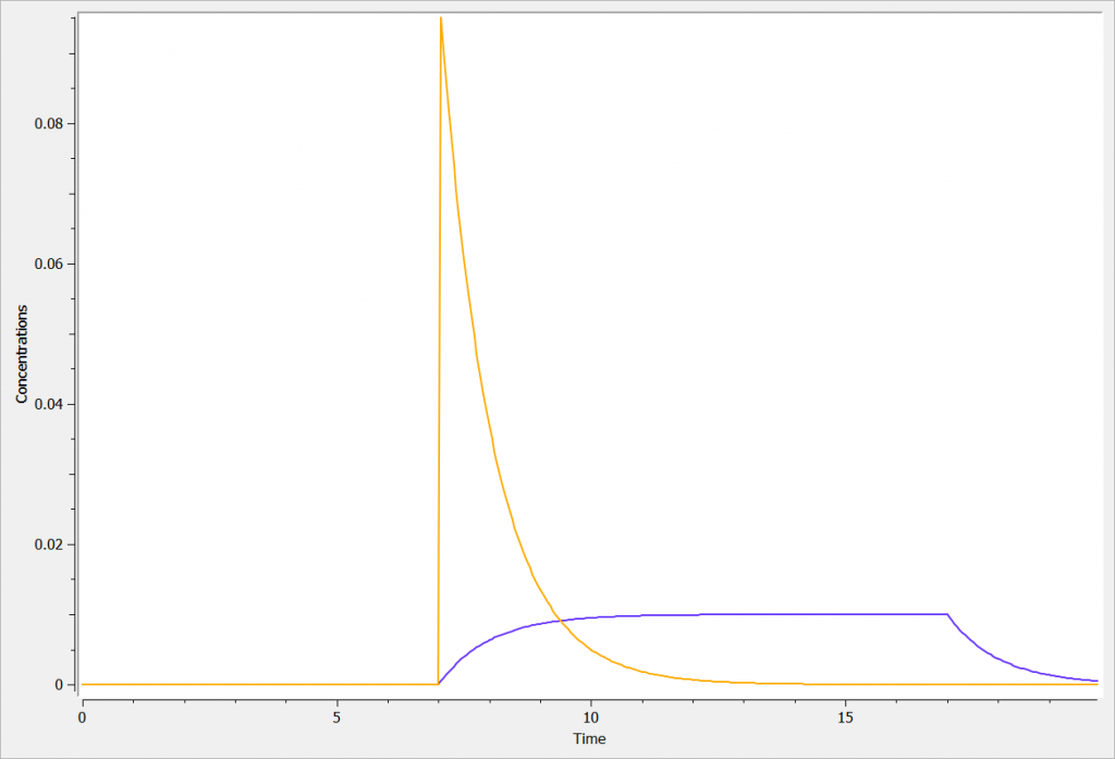
In the following example, a compartment is defined in the PK: bloc and the dynamics of the amount is defined with the iv and elimination macro. The model is implemented in the file compartment.mlxplore.mlxtran available as Mlxplore demo. A snapshot of the code is shown below:
[LONGITUDINAL]
input = {V, k}

PK:
compartment(cmt=1, amount=Ac, concentration=Cc, volume=V)
iv(cmt=1, type=1)
elimination(cmt=1, k)
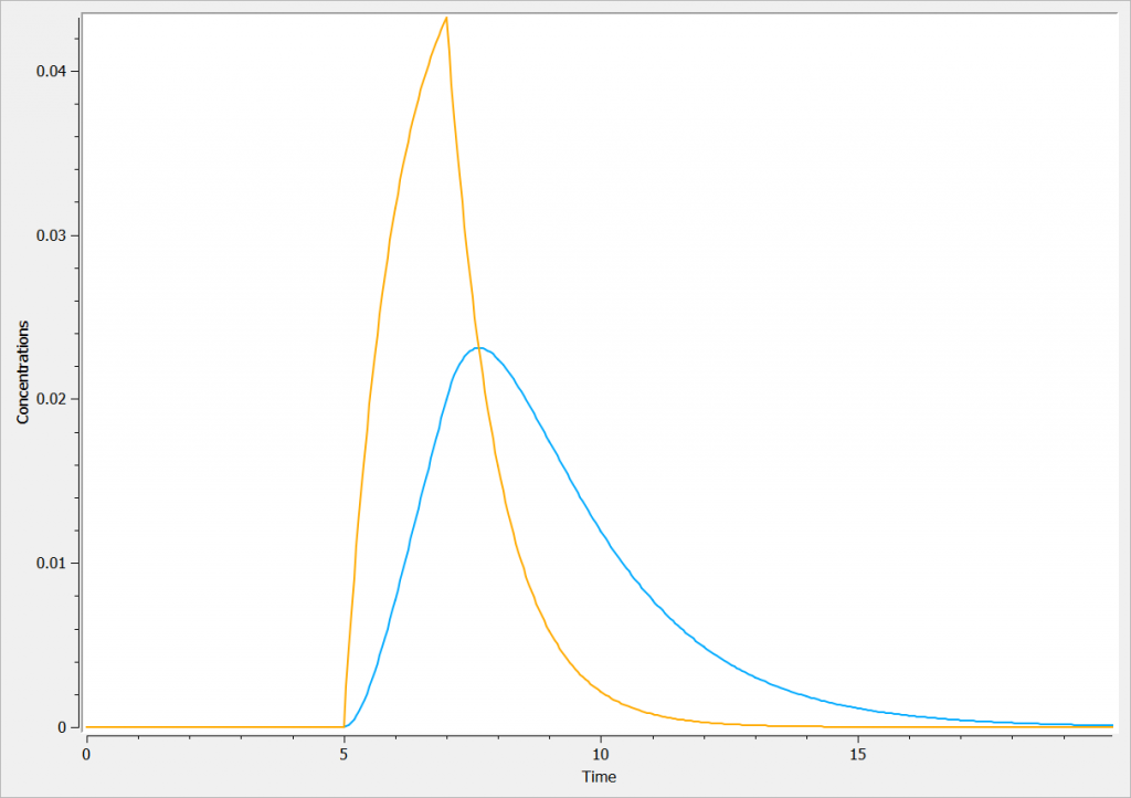
The considered administration is a dose of 1 at time 5. We defined the one compartment, and the associated concentration, amount, id, are defined in it. Therefore, it is very simple to define the associated dynamics. We added an absorption process as a bolus and defined a linear elimination. The results can be seen in the following figure.
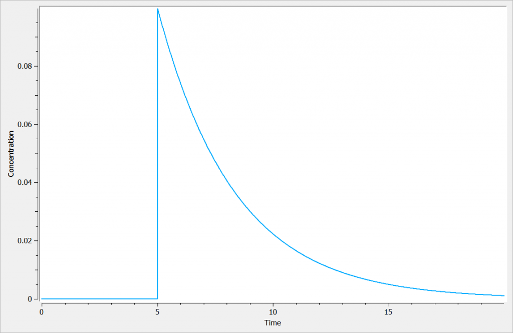
The main interest of this example is that all the parameters of the compartments are well defined and therefore their manipulation is easy.
Rules and Best Practices
- We encourage the user to use all the fields in the macro to guarantee non confusion between concentration, amount, …
CAUTION: if the volume is not given, it will be assumed to be equal to 1. The volume is in particular needed to calculate k from the clearance when Cl is used as input of the elimination macro. - The compartment definition has to be done in the first place before additional macros.
- Format restriction (non compliance will raise an exception)
- The value after cmt= is necessarily an integer.
- The value after amount=, volume= and concentration= are necessarily strings.
3.2.Peripheral macro
Purpose
The peripheral macro defines a peripheral compartment. It is equivalent to a compartment with two transfers of drug amount towards and from another base compartment. This base compartment must have been previously defined and referenced by its label. If the amount or concentration of the peripheral compartment are not outputted, then they do not need to be defined.
Arguments
Arguments for macro peripheral are:
- kij or ki_j: Input rate from the compartment of label i. It also defines a label j for the peripheral compartment. Here, both labels i and j must be integers. If i and/or j are larger than 9, the syntax with the underscore is necessary. Mandatory.
- kji or kj_i: Output rate to the compartment of label i. It also defines a label j for the peripheral compartment. Here, both labels i and j must be integers. If i and/or j are larger than 9, the syntax with the underscore is necessary. Mandatory.
- amount: Name of variable defined as the amount within the compartment. Its dynamics are defined by dose absorptions, eliminations, and the transfer rates with other compartments. These dynamics can extend an ODE system that defines a component with this name.
- volume: Name of predefined variable to use as the volume of the compartment. It enables to define concentration. The default value is 1. If the volume is not defined, the concentration cannot be defined.
- concentration: Name of the variable defined as the concentration within the peripheral compartment.
Example
PK:
; definition of a peripheral compartment with cmt=2 with rates k12 and k21,
; an amount called Ap, a volume V2, and a concentration Cp
peripheral(k12, k21, amount=Ap, volume=V2, concentration=Cp)
; definition of a peripheral compartment with cmt=3, linked to compartment 1,
; with rates k13 and k31 a volume equals by default to 1
peripheral(k13, k31)
; with compartments numbers larger than 9
peripheral(k2_13, k13_2)
Rules and best practices
- To use inter-compartment clearance Q and peripheral volume V2 as parameters instead of k12 and k21, the syntax is:
peripheral(k12=Q/V, k21=Q/V2)
- We encourage the user to use all the fields in the macro to guarantee non confusion between concentration, amount, …
- Format restriction (non compliance will raise an exception)
- The values after k are necessarily an integer (related to predefined compartment id).
- The value after kij= can be either a double or replaced by an input parameter. Calculations are not supported.
- The value after amount= and concentration= are necessarily strings.
- The value after volume= can be either a double or replaced by an input parameter. Calculations are not supported.
3.3.Effect macro
Purpose
The macro effect defines an effect compartment. The effect compartment is linked to a parent compartment. The drug exchange between the effect compartment and the parent compartment does not affect the mass balance of the parent compartment. The parent compartment must be defined before the effect compartment is defined.
Arguments
Arguments for the macro effect are:
- cmt: Label of the linked base compartment. Its default value is 1.
- ke0: Transfer rate from the linked base compartment. Mandatory.
- concentration: Name of the variable defined as the concentration within the effect compartment. Mandatory.
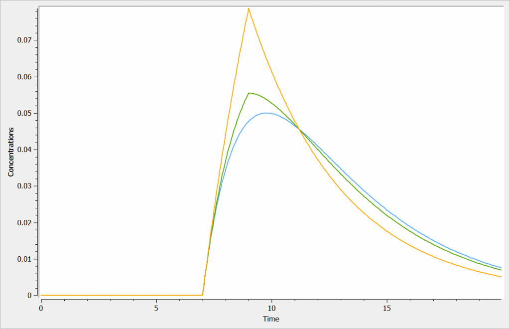
Example:
PK:
; Define an effect compartment linked to the base compartment 1,
; with a transfer rate ke0 to the effect compartment,
; with Ce as concentration's name
effect(cmt=1, ke0, concentration=Ce)
Example with Mlxplore:
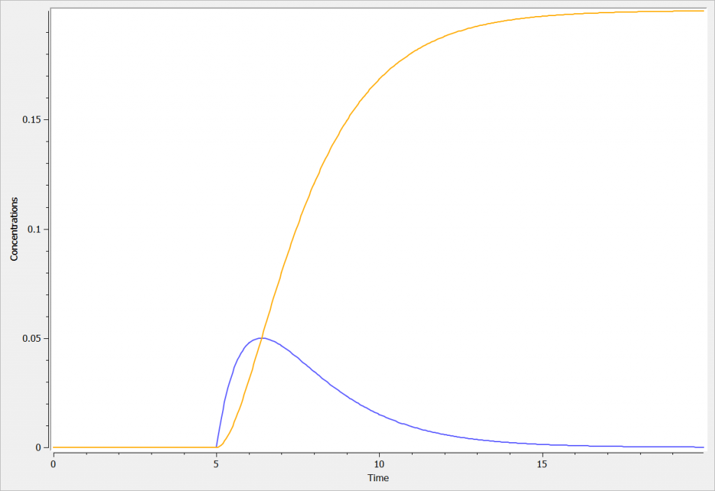
In the following example, a compartment is defined in the PK: bloc. An iv absorption process along with a linear elimination process is added to the main compartment. An effect is added with a transfer rate ke0. The model is implemented in the file effect.mlxplore.mlxtran available in the Mlxplore demos. The code is detailed below:
<MODEL>
[LONGITUDINAL]
input = {V, k, ke0}

PK:
compartment(cmt=1, amount=Ac, concentration=Cc, volume=V)
elimination(cmt=1, k)
iv(cmt=1)
effect(cmt=1, ke0, concentration=Ce)

<DESIGN>
[ADMINISTRATION]
admin = {time=5, amount=1, target=Ac, rate=.5}

<PARAMETER>
V = 10
ke0  = .5
k = 1

<OUTPUT>
grid = 0:.05:20
list = {Ce,Cc}

<RESULTS>
[GRAPHICS]
p = {y={Ce, Cc}, ylabel='Concentrations', xlabel='Time'}
The concentration in the base compartment and in the effect compartment are proposed in the following figure where the concentration in the main (base) compartment is in orange, and the one in the effect compartment is in blue.
Rules and Best Practices:
- We encourage the user to use all the fields in the macro to guarantee non confusion between fields.
- A base compartment must be defined first.
- Format restriction (non compliance will raise an exception)
- The value after cmt= is necessarily an integer.
- The value after ke0= can be either a double or replaced by an input parameter. Calculations are not supported.
- The value after concentration= is necessarily a string.
3.4.Transfer macro
Purpose
The macro transfer defines a uni-directional transfer process from a base compartment to a target compartment. The base compartment and the target compartment must be defined first before the transfer can be defined. For the more common bi-directional transfer process it is better to use the macro peripheral instead of the macro transfer, in particular as it allows to use the analytical solution, which is not the case with the macro transfer.
Arguments
Its named arguments are:
- from: Label of the source compartment for the transfer. Its default value is 1.
- to: Label of the target compartment for the transfer. Its default value is 1.
- kt: Rate of the transfer. Mandatory.
Example
PK:
; transfer from compartment 1 to compartment 2 with a rate kt
transfer(from=1, to=2, kt)
Example with Mlxplore:
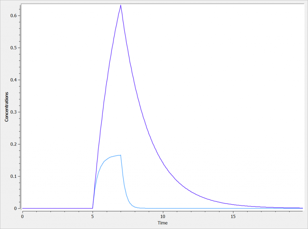
In the following example, two compartments are defined in the PK: block. A transfer from compartment 1 to compartment 2 is added, with a transfer rate kt. The model is implemented in the file transfer.mlxplore.mlxtran available in the Mlxplore demos, and shown below:
<MODEL>
[LONGITUDINAL]
input = {V1, V2, kt}

PK:
compartment(cmt=1, amount=Ac, concentration=Cc1, volume=V1)
compartment(cmt=2, amount=Ad, concentration=Cc2, volume=V2)
oral(cmt=1,ka=1)
transfer(from=1, to=2, kt)

<DESIGN>
[ADMINISTRATION]
admin = {time=5, amount=1, target=Ac, rate=.5}

<PARAMETER>
V1 = 10
V2 = 5
kt = .5

<OUTPUT>
grid = 0:.05:20
list = {Cc1,Cc2}

<RESULTS>
[GRAPHICS]
p = {y={Cc1, Cc2}, ylabel='Concentrations', xlabel='Time'}
The concentration in the compartment and the transfer are shown in the following figure in blue and orange respectively.
Best Practices:
- We encourage the user to use all the fields in the macro to guarantee non confusion between the fields.
- Format restriction (non compliance will raise an exception)
- The value after from= and to= are necessarily integers.
- The value after kt= can be either a double or replaced by an input parameter. Calculations are not supported.
3.5.Depot macro
Description
The macro depot is a multipurpose macro that can accommodate different types of administrations. It is typically used together with ODE systems to define how the administrations from the data set are linked with the model variables. It is the only macro that can be used with ODEs for administration without defining a compartment. With the macro depot, a bolus, an infusion (with INFUSION RATE or INFUSION duration defined in the data set), a zero order absorption, or a first order absorption (with or without transit process) can be defined.
We encourage the user to use all the fields in the macro to guarantee no confusion between parameters.
As for other macros, depot must be used in a block PK:, while ODEs must be defined in a block EQUATION:.
Arguments
The depot macro can be used for bolus doses, infusions (with INFUSION RATE or INFUSION duration defined in the data set), zero-order absorptions, and first-order absorptions. Some arguments are common for the three types of administrations, some are specific.
The arguments common to bolus, zero-order and first-order absorption are:
- adm: Administration type of doses subject to the absorption process. Its default value is 1. Alias: type. Thus, when defining a treatment in Mlxplore for example, instead of defining a target, the user should define a type and apply the dedicated absorption process on it.
- target: Name of the ODE variable that is targeted by the administration. Mandatory.
- Tlag: Lag time before the absorption. Its default value is 0.
- p: Fraction of the absorbed amount. It can affect the effective rate of the absorption, not its duration. p can take any positive value (including > 1). Its default value is 1.
Specific arguments for bolus doses:
For bolus doses, no additional argument is needed.
The following code defines a bolus for doses of type 1 (e.g ADM=1 in the data set), applied to the ODE variable Ad, with a delay Tlag and a fraction absorbed F :
PK:
depot(type=1, target=Ad, Tlag, p=F)
Specific arguments for zero-order absorption (i.e infusion):
To define a zero-order absorption, the following argument must be added:
- Tk0: Duration of the zero order absorption. Mandatory to define zero-order absorption.
The following code defines a zero-order absorption process of duration Tk0, for doses of type 2, applied to the ODE variable Ac, without lag time (Tlag=0 when not specified) and with the entire dose being absorbed (p=1 when not defined):
PK:
depot(type=2, target=Ac, Tk0)
Specific arguments for first-order absorption:
To define a first-order absorption, the following arguments can be added:
- ka: Rate of the first order absorption. Mandatory to define first-order absorption.
- Ktr: Transit rate.
- Mtt: Mean transit compartments time for the absorption.
The following code defines a first-order absorption process with rate ka, for doses of type 1 (type=1 when not specified), applied to the ODE variable Ac, with a lag-time Tlag of 2.1, and only 30% of the dose being absorbed:
PK:
depot(target=Ac, ka, Tlag=2.1, p=0.3)
Note: In case of transit compartments and multiple doses, the amounts in the depot, transit and absorption compartments are reset at each new doses. Thus the implementation is valid only if the dose is fully absorbed before the next dose administration. The amount in the central (and possibly other compartments) is not reset and can accumulate.
Rules
- The value after type= must be an integer.
- The value after target= must be a string representing the ODE variable
- The inputs after Tlag=, p=, Tk0=, ka=, Ktr=, Mtt= can be either a
- Double
- Input parameter
- Variable
- Calculations are not supported
- The associated treatment or administration can be defined with a rate or an infusion timing from the data set (RATE and TINF column-types in the data set). The rules are the same as for the iv macro.
3.6.Absorption/oral macro
Purpose
The macro absorption/oral enables to link the administration and the model, for zero-order and first-order absorption processes (for bolus administrations, use the iv macro instead). For Mlxtran the macro names ‘absorption’ and ‘oral’ can be used interchangeably. The administration can either be defined in a data set when Monolix is used, or the administration can be defined via an administration design definition when Mlxplore or Simulx are used. In order to handle models with several administrations each administration has a unique identifier called adm. This identifier must be defined in the data set or in the administration design definition, and used in the absorption/oral macro.
Arguments
The absorption/oral macro can be used for zero-order and first-order absorptions. The arguments common to the two absorptions are:
- adm: Administration type of doses subject to the absorption process. Its default value is 1. Alias: type. Thus, when defining a treatment in Mlxplore for example, instead of defining a target, the user should define an administration type and apply the dedicated absorption process on it.
- Tlag: Lag time before the absorption. Its default value is 0.
- p: Final proportion of the absorbed amount. It can affect the effective rate of the absorption, not its duration. p can take any positive value (including > 1). Its default value is 1.
- cmt: Label of the compartment called in by the absorption process. Its default value is 1.
To define a zero-order or first-order absorption, the additional arguments defined below are needed.
Arguments specific to a zero-order absorption (i.e infusion)
To define a zero-order absorption, the following argument must be added:
- Tk0: Duration of the zero order absorption. Mandatory to define a zero-order absorption.
Example:
; zero order absorption process for the doses of type 1, in compartment 1 with a delay Tlag of 1 and a duration Tk0
absorption(adm=1, cmt=1, Tlag=1, Tk0 = 2, p=1)
Arguments specific to a first-order absorption
To define a first-order absorption, the following arguments can be added:
- ka: Rate of the first order absorption. Mandatory to define a first-order absorption.
- Ktr: Transit rate.
- Mtt: Mean transit time for the absorption.
Example:
PK:
; first order absorption process for the doses of type 1, in compartment 1 with a delay Tlag of 1 and a rate ka
absorption(type=1, cmt=1, Tlag=1, ka)
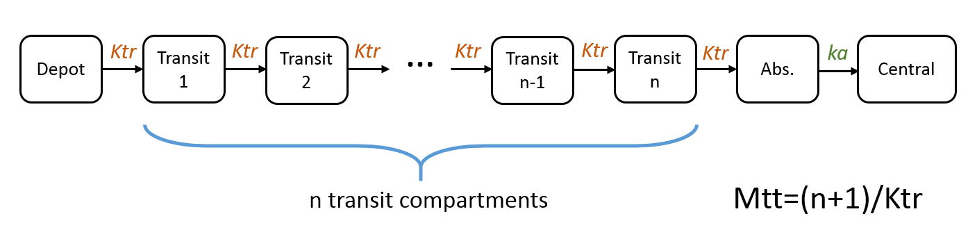
Note: in case of transit compartments, the mean transit time is defined as Mtt = (n+1)/Ktr with n the number of transit compartments (excluding the depot compartment and the absorption compartment):
The implementation is the same as described in Savic et al, “Implementation of a transit compartment model for describing drug absorption in pharmacokinetic studies” (2007), except that to approximate the factorial n!, we use the gamma function, which is more precise, instead of the Stirling formula.
In case of multiple doses, we assume that the previous dose has been completely absorbed (i.e concentration is the Abs compartment is almost zero) when the next dose is administered. If this is not the case, the remaining concentration in the Abs compartment is erased when the next dose is applied, leading to a loss of dose amount entering the system.
Example with mixed absorptions
Some drugs can exhibit atypical absorption profiles with for instance a zero-order absorption followed by a first-order absorption, or first and zero-order simultaneously.
Sequential absorption, zero-order followed by first-order
In the example below, a fraction F1 of the drug is absorbed via a zero-order process for a duration Tk0. The remaining fraction 1-F1 is then absorbed via a first-order process, which starts with a lag-time Tk0 (i.e at the end of the zero-order absorption phase).
PK:
absorption(adm=1, cmt=1, Tk0, p=F1)
absorption(adm=1, cmt=1, ka, p=1-F1, Tlag=Tk0)
Simultaneous first-order and zero-order absorption
In the example below, a fraction F1 of the drug is absorbed via a first-order process (with absorption rate ka). Simultaneously the remaining fraction 1-F1 is absorbed via a zero-order process.
PK:
absorption(adm=1, cmt=1, ka, p=F1)
absorption(adm=1, cmt=1, Tk0, p=1-F1)
A lag time for one or the other process can be added if necessary.
Example with Mlxplore: Comparison of absorptions
In the presented example, we show the difference between the two absorption processes. In addition, the effect of the Ktr and Mtt parameters is explored in a third model. The model is implemented in the following file mlxplore_Absorption.txt.
<MODEL>
[LONGITUDINAL]
input = {V, Tlag, ka, Tk0, Ktr, Mtt}

PK:
compartment(cmt=1, amount=A1, concentration=Cc_zoa, volume=V)
absorption(cmt=1, adm=1, Tk0)
elimination(cmt=1, k=1)

compartment(cmt=2, amount=A2, concentration=Cc_foa, volume=V)
absorption(cmt=2, adm=1, Tlag, ka)
elimination(cmt=2, k=1)

compartment(cmt=3, amount=A3, concentration=Cc_foaT, volume=V)
absorption(cmt=3, adm=1, Tlag, ka, Ktr, Mtt)
elimination(cmt=3, k=1)

EQUATION:
ddt_A1 = 0
ddt_A2 = 0
ddt_A3 = 0

<DESIGN>
[ADMINISTRATION]
adm = {time=5, amount=1, adm=1}

<PARAMETER>
V = 10
Tlag = 2
ka = .5
Tk0 = 2
Ktr = 3
Mtt = 2

<OUTPUT>
grid = 0:.05:20
list = {Cc_zoa, Cc_foa, Cc_foaT}

<RESULTS>
[GRAPHICS]
p = {y={Cc_zoa, Cc_foa, Cc_foaT}, ylabel='Concentrations', xlabel='Time'}
The three concentrations are presented in the following figure.
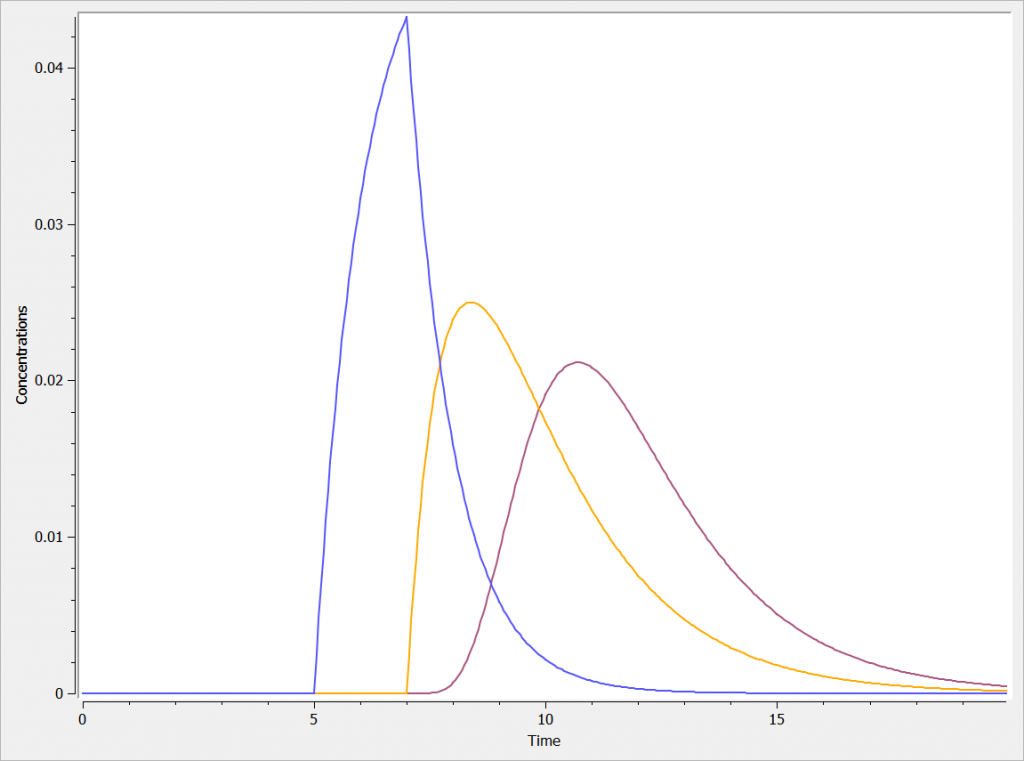
One can clearly see the differences between the zero order absorption (Cc_zoa in blue), the first order absorption (Cc_foa in orange) and the absorption with transit compartments (in purple).
Rules and Best Practices:
- We encourage the user to use all the fields in the macro to guarantee no confusion between parameters
- Format restriction (non compliance will raise an exception)
- The value after cmt= and type= are necessarily integers.
- The value after Tlag=, p=, V=, ka=, Tk0=, Ktr=, Mtt= can be either a double or replace by an input parameter. Calculations are not supported.
- The associated treatment or administration can not be defined with a rate nor an infusion timing (RATE and TINF column-types in the data set). If a rate or an infusion timing is present, the user can use the iv macro and/or define a compartment to define the dynamics of the absorption.
3.7.IV macro
Purpose
The macro iv enables to link the administration with the model, for intravenous doses (bolus or infusion). Doses defined in the [ADMINISTRATION] section or in the data set without an administration rate or infusion time are instantaneously absorbed within the associated compartment, as an IV bolus. Doses with an administration rate or infusion time (e.g keyword ‘rate’ in the [ADMINISTRATION] section of a Mlxplore file, or column-type RATE or TINF in the data set) are absorbed according to a zero order process, as an IV infusion.
Arguments
Arguments for macro iv are:
- cmt: Label of the compartment called in by the absorption process. Its default value is 1.
- adm: Administration type of doses subject to the absorption process. Its default value is 1. Alias: type. Thus, when defining a treatment in Mlxplore for example, instead to define a target, the user should define a type and apply the dedicated absorption process on it.
- Tlag: Lag time before the absorption. Its default value is 0.
- p: Final proportion of the absorbed amount. It can affect the effective rate of the absorption, not its duration. p can take any positive value (including > 1). Its default value is 1.
Example:
PK; intravenous bolus for the doses of type 1, in compartment 1 with a delay Tlag at 1
iv(adm=1, cmt=1, Tlag=1, p=1)
Example with Mlxplore
In the presented example, we show the difference two iv processes with and without a rate in the administration.
<MODEL>
[LONGITUDINAL]
input = {V, Tlag}

PK:
compartment(cmt=1, amount=A1, concentration=Cc_iv_bolus, volume=V)
iv(cmt=1, adm=1, Tlag)
elimination(cmt=1, k=1)

compartment(cmt=2, amount=A2, concentration=Cc_iv_inf, volume=V)
iv(cmt=2, adm=2, Tlag)
elimination(cmt=2, k=1)

<DESIGN>
[ADMINISTRATION]
adm_1 = {time=5, amount=1, adm=1}
adm_2 = {time=5, amount=1, adm=2, rate=.1}

<PARAMETER>
V = 10
Tlag = 2

<OUTPUT>
grid = 0:.05:20
list = {Cc_iv_bolus, Cc_iv_inf}

<RESULTS>
[GRAPHICS]
p = {y={Cc_iv_bolus, Cc_iv_inf}, ylabel='Concentrations', xlabel='Time'}
The two concentrations (Cc_iv_bolus in orange, and Cc_iv_inf in blue) are presented in the following figure.
Rules and Best Practices:
- We encourage the user to use all the fields in the macro to guarantee no confusion between parameters
- Format restriction (non compliance will raise an exception)
- The value after cmt= and adm= are necessarily integers.
- The value after Tlag=, p= can be either a double or replaced by an input parameter. Calculations are not supported.
- With the iv macro, it is not possible to give the rate or duration of the infusion as a parameter or fixed value. To do so, use the absorption macro with duration parameter Tk0 to define a zero-order absorption (i.e infusion).
- When the iv macro is used in combination with a data set with a column-type RATE:
- if RATE >0: infusion with rate RATE and duration AMT/RATE
- if RATE <=0: bolus
- When the iv macro is used in combination with a data set with a column-type TINF:
- if TINF >0: infusion of duration TINF at a rate AMT/TINF
- if TINF <=0: bolus
3.8.How to play with bioavailabiliy ?
Purpose
The bioavailability parameter p, available in the administration macros (‘depot’, ‘absorption’, and ‘iv’), defines the fraction of dose absorbed by the administration type.
The bioavailability parameter can also be used to perform a unit conversion between the amount provided in the data set and the quantities represented in the model (for instance from mg to mmol). For this usage, p can take values greater than 1.
Example
In the following example, we compare a zero-order absorption process, a first-order absorption process, and a process with mixed zero and first-order absorptions.
<MODEL>
[LONGITUDINAL]
input = {V, Tlag, ka, Tk0, F}

PK:
compartment(cmt=1, amount=A1, concentration=Cc_zoa, volume=V)
absorption(cmt=1, type=1, Tlag, Tk0, p=1)
elimination(cmt=1,k=.25)

compartment(cmt=2, amount=A2, concentration=Cc_foa, volume=V)
absorption(cmt=2, type=1, Tlag, ka, p=1)
elimination(cmt=2,k=.25)

compartment(cmt=3, amount=A3, concentration=Cc_mixed, volume=V)
absorption(cmt=3, type=1, Tlag, Tk0, p=F)
absorption(cmt=3, type=1, Tlag, ka, p=1-F)
elimination(cmt=3,k=.25)

<DESIGN>
[ADMINISTRATION]
adm = {time=5, amount=1, type=1}

<PARAMETER>
V = 10
Tlag = 2
ka = .5
Tk0 = 2
F = .25

<OUTPUT>
grid = 0:.05:20
list = {Cc_zoa Cc_foa, Cc_mixed}

<RESULTS>
[GRAPHICS]
p = {y={Cc_zoa Cc_foa, Cc_mixed}, ylabel='Concentrations', xlabel='Time'}
The zero-order absorption is shown in orange, the first-order absorption in blue and the mixed one in green, in the figure below:
3.9.Elimination macro
Purpose
The elimination macros permits to define different elimination processes (linear or Michaelis-Menten) for compartments. Several eliminations can be defined for the same compartment.
Arguments
Some arguments are common to the two elimination types, while some are specific to a linear or to a Michaelis-Menten type of elimination.
The arguments that are common to linear and Michaelis-Menten are:
- cmt: Label of the compartment emptied by the elimination process. Its default value is 1.
- V: Volume involved in the elimination process. When not specified, its default value is the volume of the compartment defined by cmt.
Additional arguments are needed to define a linear or Michaelis-Menten elimination type.
Arguments specific to a linear elimination
The use of one of the following additional arguments defines a linear elimination:
- k: Rate of the elimination.
- Cl: Clearance of the elimination.
Only one of k or Cl must be defined.
Note, that if no volume has been defined for the compartment and no volume has been defined for the elimination process, then the default volume V=1 is assumed.
Example:
PK:
elimination(cmt=1,k)
Arguments specific to a Michaelis-Menten elimination
The use of both of the following additional arguments defines a Michaelis-Menten elimination:
- Vm: Maximum elimination rate. The unit of Vm is amount/time.
- Km: Michaelis-Menten constant. The unit of Km is a concentration.
Both arguments must be defined.
Example:
PK:
elimination(cmt=1, Vm, Km)
Example with Mlxplore : Comparison of the two eliminations
In the following example, the difference between the two elimination processes is demonstrated. The model is implemented in the file elimination.mlxplore.mlxtran, available in the Mlxplore demos and shown below:
<MODEL>
[LONGITUDINAL]
input = {k, Vm, Km}

PK:
compartment(cmt=1, amount=Alin, concentration=Cc_lin)
elimination(cmt=1, k)
iv(cmt=1, adm=1)

compartment(cmt=2, amount=AMM, concentration=Cc_MM)
elimination(cmt=2, Vm, Km)
iv(cmt=2, adm=2)

<DESIGN>
[ADMINISTRATION]
adm_lin = {time=5, amount=1, adm=1, rate=.5}
adm_MM = {time=5, amount=1, adm=2, rate=.5}

<PARAMETER>
k  = .5
Vm  = 2
Km = .5

<OUTPUT>
grid = 0:.05:20
list = {Cc_lin,Cc_MM}

<RESULTS>
[GRAPHICS]
p = {y={Cc_lin,Cc_MM}, ylabel='Concentrations', xlabel='Time'}
The two concentrations are presented in the following figure, with the linear elimination in purple and the Michaelis-Menten elimination in light blue.
One can clearly see the nonlinearities in the Michaelis-Menten elimination process.
Example: PK model with dual elimination pathways
The following model implemented with PK macros includes two compartments, an oral absorption and a dual elimination pathway with parallel linear and Michaelis-Menten eliminations. An equivalent model, implemented with ODEs, is defined in the TMDD model library: it corresponds to the Michaelis-Menten approximation of a TMDD model.
[LONGITUDINAL]
input = {ka, V, Vm, Km, Cl, Q, V2}

PK:
kel = Cl/V
k12 = Q/V
k21 = Q/V2
compartment(cmt=1, concentration=Cc, volume=V)
absorption(cmt=1, ka)
peripheral(k12, k21)
elimination(cmt=1, k=kel)
elimination(cmt=1, Vm, Km)

OUTPUT:
output={Cc}
Rules and Best Practices:
- We encourage the user to use all the fields in the macro to guarantee no confusion between parameters
- Format restriction (non compliance will raise an exception)
- The value after cmt= is necessarily an integer.
- The value after V=, k=, Cl=, Km=, Vm= can be either a double or be replaced by an input parameter. Calculations are not supported.
3.10.Empty and reset macros
Description
The macro empty can be used to set any component of the system, defined in an ODE, to 0 at any given time. Similarly, the macro reset is used to reset a variable of the system to its initial value. Empty or reset times are indicated via a type of administration. The actions of these macros are thus selective, contrary to the reset applied with an EVID column in the dataset with values 3, which resets all compartments.
Arguments
The arguments are the same for both empty and reset macros:
- adm: Administration type used to indicate empty or reset times. Its default value is 1. Alias: type. The empty and reset macrso only use the administration times, not the amounts.
- target: Name of the ODE variable that is set to 0 or reset to its initial value at the specified times, or target=all to reset all system variables. Mandatory.
The following code defines an emptying of the ODE variable Ap on administration times of type 1 (e.g ADM=1 in the data set).
PK:
empty(adm=1, target=Ap)
PK:
depot(adm=1, target=Ap, p=-Ap/amtDose)
The following code defines a reset based on administration times of type 2 (e.g ADM=2 in the data set), applied to the ODE variable Ac.
PK:
reset(adm=2, target=Ac)
PK:
empty(adm=3, target=Ac)
empty(adm=3, target=Ap)
PK:
reset(adm=3, target=all)
Rules
- The value after type= or adm= must be an integer.
- The value after target= must be a string representing the ODE variable.
Empty example: urine compartment
When using this model with a data set, urine would be collected over consecutive periods of 12 hours and the amount of drug measured in the urine volume collected for each period would be recorded.
<MODEL>

[LONGITUDINAL]
input = {ka, Cl, V1, Q, V2, p_urine}

PK:
k_urine = p_urine*Cl/V1
k_non_urine = (1-p_urine)*Cl/V1
k12 = Q/V1
k21 = Q/V2

; Dose administration to central compartment (plasma)
depot(adm=1, target=Ac, ka)

; Reset of urine compartment
reset(adm=2, target=Aurine)

EQUATION:
t_0=0
Ac_0=0
Ap_0=0
Aurine_0=0

ddt_Ac = - k_non_urine*Ac - k12*Ac + k21*Ap - k_urine*Ac
ddt_Ap = k12*Ac-k21*Ap
ddt_Aurine = k_urine*Ac

Cc=Ac/V1

OUTPUT:
output = {Cc, Aurine}

<PARAMETER>
Cl =0.5
Q =1
V1 =5
V2 =8
ka =10
p_urine =0.05

<DESIGN>

[ADMINISTRATION]
adm1_1={ type=1,time={0}, amount={10} }
adm2_1={ type=2,time={1,13,25,37,49,61,73,85,97}, amount={1,1,1,1,1,1,1,1,1} }

[TREATMENT]
treatment1={adm1_1,adm2_1}

<OUTPUT>
grid=0.02:0.1:100
list={Cc,Aurine}
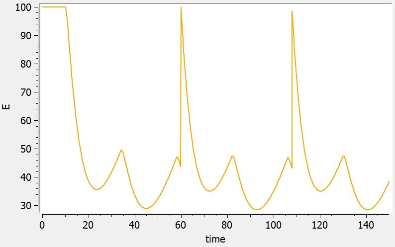
Reset example: PD variable
<MODEL>
[LONGITUDINAL]
input = {ka, k, E0, IC50, kout}

PK:
depot(target=Ad, type=1)
reset(target=E, type=2)

EQUATION:
E_0 = E0
kin = E0*kout

ddt_Ad = -ka*Ad
ddt_Ac = ka*Ad - k*Ac
ddt_E = kin*(1 - Ac/(Ac+IC50)) - kout*E

OUTPUT:
output = {E}

<PARAMETER>
ka=0.3
k=0.1
E0=100
IC50=20
kout=0.2

<DESIGN>
[ADMINISTRATION]
adm1 = { type=1,time=10:24:136, amount={100} }
adm2 = { type=2,time=60:48:136, amount={1} }

[TREATMENT]
treatment1={adm1, adm2}

<OUTPUT>
grid=0:0.1:150
list={E}
3.11.Overview of macro input elements
Purpose
The goal is to propose an overview of macro input elements as proposed in the following table.
Several points have to be noticed
- Macros are used in the PK: section of the Mlxtran model
- Parameters for a macro call are matched by name, not by ordering
- Default values are given in brackets: for example (0)
- Before concentrations can be used the volumes MUST be defined
- adm and type are equivalent
| Macro input parameters | Macros | ||||||||
| Administration | Compartment | Process | |||||||
| Macro | depot | iv | oral or absorption | compartment | elimination | peripheral | transfer | effect | |
| Identifier | adm (1) | adm (1) | adm (1) | cmt(1) | |||||
| Target | target | cmt(1) | cmt(1) | cmt(1) | target compartments are defined by indices | from(1) to (1) | cmt(1) | ||
| Rates | Required | ka or Tk0 | k or Cl or Vm, Km | (k12, k21), (kij, kji) or (k_i_j, k_j_i) | kt | ke0 | |||
| Optional | ka or Tk0 Tlag (0) Ktr, Mtt (0) |
Tlag (0) | Tlag (0) or Mtt (0), Ktr |
(k13, k31) (k23, k32) |
|||||
| Bioavailability of fraction of the dose absorbed | p (1) | p (1) | p (1) | ||||||
| Volume | volume (1) | volume (1) | |||||||
| Concentration | concentration | concentration | concentration | ||||||
| Amounts | amount | amount | |||||||
| Explanation | No need to define compartments. Used with ODEs |
Target compartment must be defined first Rate or Tinf are taken from data set |
Target compartment must be defined first | Defines compartment and process at the same time | |||||
3.12.Overview of PK model input parameters
| Pkmodel function input | Process | Required parameter | Optional parameter | Excluded parameter |
| Administration | Bolus | Tlag, p | Tk0, ka, Ktr, Mtt | |
| Zero order absorption | Tk0 | Tlag, p | ka, Ktr, Mtt | |
| First order absorption | ka | Tlag, p | Tk0 | |
| Absorption with transit compartments of mean transit time Mtt and transit rate Ktr | ka, Ktr, Mtt | Tlag, p | Tk0 | |
| Bioavailability; fraction of the dose absorbed | p | Tlag | Tk0, ka, Ktr, Mtt | |
| Compartment | Volume | V | ||
| Elimination | Linear, rate | ka | Cl, Km, Vm | |
| Linear, clearance | Cl | k, Km, Vm | ||
| Michaelis Menten | Km, Vm | K, Cl | ||
| Transfers | Transfer rates | (k12,k21) (k13, k31 ) |
||
| Effect compartment transfer rate constant | ke0 | |||
| Output | Concentration in the central compartment | first output name | ||
| Concentration in the effect compartment | second output name |
4.pkmodel
Introduction
The function pkmodel permits to define common PK models in a very concise way. The purpose of this macro is to simplify the modeling of classical pharmacokinetics. The PK model is inferred from the provided set of named arguments. Most of the arguments are optional, and the pkmodel function enables several parametrizations, to select different models of absorption, elimination, etc. With the pkmodel function, the most common PK models are available. The concentration within the central compartment is the main output of the function. If an effect compartment is defined, its concentration defines the second output. The administration of the doses is always supposed to be of type 1, and the default absorption is the IV bolus one. The label of the central compartment is 1. The pkmodel function can also be used within the block EQUATION: or the block PK:.
We first give typical examples and then list all possible arguments.
Examples
Example 1: One compartment model with intravenous (bolus or infusion) administration
Cc = pkmodel(V, Cl)
This simple set of named arguments for pkmodel defines a PK model with one central compartment of label 1, with the default intravenous bolus administration for doses of administration type 1 and a linear elimination with the clearance parametrization in Cl. The volume of the central compartment is V. The concentration in the central compartment is the output Cc of the function.
If a column is tagged as infusion duration or as infusion rate in the data, this is recognized by the pkmodel macro and the doses of administration type 1 with a non-empty infusion rate or duration are administered as an infusion instead of a bolus.
Example 2: Two-compartment model with first order absorption with lag time
- With elimination rates: parameters Tlag, ka, V, k, k12, k21
Cc = pkmodel(Tlag, ka, V, k, k12, k21)
- With clearances: parameters Tlag, ka, V, Cl, Q, V2
Cc = pkmodel(Tlag, ka, V, k=Cl/V, k12=Q/V, k21=Q/V2)
Note that it is not possible to give Q and V2 as direct input parameters. Instead, we give the recognized keywords k12 and k21, and defined them using Q, V and V2.
Example 3: Three-compartment model with zero-order absorption
Cc = pkmodel(Tk0, V, k, k12, k21, k13, k31)
Tk0 represents the duration of the zero-order absorption. k12 and k21 are the rates to and from the first peripheral compartment and k13 and k31 are the rates to and from the second peripheral compartment.
Example 4: One compartment model with transit compartments
Cc = pkmodel(ka, Mtt, Ktr, V, Cl)
In case of transit compartments, the mean transit time is defined as Mtt = (n+1)/Ktr with n the number of transit compartments (excluding the depot compartment and the absorption compartment) and Ktr the transit rate.
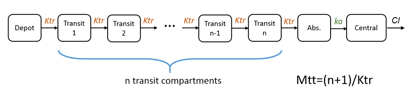 The implementation is the same as described in Savic et al, “Implementation of a transit compartment model for describing drug absorption in pharmacokinetic studies” (2007), except that to approximate the factorial n!, we use the gamma function, which is more precise, instead of the Stirling formula.
Note that this model has no analytical solution, so the ODE system is used.
Example 5: One compartment model with effect compartment
{Cc, Ce} = pkmodel(ka, V, Cl, ke0)
The one-compartment model is connected to an effect compartment with a bi-directional rate ke0. The concentration in the effect compartment is called Ce in this example and can for instance be used to define a PD model.
Example 6: Model using almost all arguments
{Cc, Ce} = pkmodel(Tlag, ka, p, V, Vm, Km, k12, k21, k13, k31, ke0)
This more complex set of named arguments for pkmodel defines a PK model of one central compartment, with a first order absorption of rate ka for doses of administration type 1, and a Michaelis-Menten elimination of parameters Vm and Km. The volume of the central compartment is V. The concentration in the central compartment is the first output Cc of the function. An effect compartment is defined with a rate ke0 and its concentration is the second output Ce. Two peripheral compartments of labels 2 and 3 are linked to the central compartment of label 1. The respective couples of exchange rates are (k12, k21) and (k13, k31). The first order absorption has a lag time Tlag and the absorbed amount is scaled with a proportion of p.
List of arguments
The complete set of named arguments and output for pkmodel follows. They belong to the central compartment, the absorption process, the elimination process, the exchanges with the peripheral compartments, or an effect compartment. Some arguments are mutually exclusive, or require other ones to be also defined. Most of them are optional, so the mandatory arguments are stated.
Arguments for the central compartment
-
- Cc = pkmodel(…): The first output is the concentration within the central compartment. Another name can be used. Mandatory.
- V: Volume of the central compartment. Mandatory.
Arguments for the absorption process of a standard PK model
-
- Tk0: Defines a zero order absorption of duration Tk0. Excludes ka, Ktr and Mtt.
- ka: Defines a first order absorption of rate ka. Excludes Tk0.
- Ktr: Along with ka and Mtt, defines an absorption with transit compartments, with transit rate Ktr. Excludes Tk0.
- Mtt: Along with ka and Ktr, defines an absorption with transit compartments, with mean transit time Mtt. Excludes Tk0.
- Tlag: Lag time before the absorption.
- p: Final proportion of the absorbed amount. Can affect the effective rate of the absorption, not its duration.
- default if no argument supplied for the absorption process: iv bolus
Arguments for the elimination process of a standard PK model
-
- k: Defines a linear elimination of rate k. Excludes Cl, Vm and Km.
- Cl: Along with V, defines a linear elimination of clearance Cl. Excludes k, Vm and Km.
- Vm: Along with V and Km, defines a Michaelis-Menten elimination of maximum elimination rate Vm. Units of Vm are amount/time. Excludes k and Cl.
- Km: Along with V and Vm, defines a Michaelis-Menten elimination of Michaelis-Menten constant Km. Units of Km are concentration so amount/volume. Excludes k and Cl.
Arguments for the peripheral compartments of a standard PK model
-
- k12: Along with k21, defines a peripheral compartment 2 of input rate k12.
- k21: Along with k12, defines a peripheral compartment 2 of output rate k21.
- k13: Along with k31, defines a peripheral compartment 3 of input rate k13.
- k31: Along with k13, defines a peripheral compartment 3 of output rate k31.
Arguments for the effect compartment of a standard PK model
-
- {Cc, Ce} = pkmodel(…): The second output is the concentration within the effect compartment. Another name can be used.
- ke0: Defines an effect compartment with transfer rate ke0 from the central compartment.
Additional possibilities
Knowing the label of the central compartment (cmt=1) and the administration type supported by the function pkmodel (type=1), one can build up a custom PK model by adding other PK elements to a base standard PK model. Referencing this label and administration type of value 1 allows to connect the additional PK elements.
Overview of arguments
Overview of input arguments for the pkmodel() macro
Rules
- Only one type of administration is allowed
- Only one pkmodel function is allowed in the Mlxtran file
- Arguments must be from the list of defined arguments for pkmodel. Arguments with different names are not recognised.
- pkmodel can not be used together with any macros for the administration. The administration is defined exclusively with the arguments supplied to pkmodel()
- A pkmodel output can be used with ODEs or with macros.
- pkmodel can also be defined in the PK: block or the EQUATION: block.
5.[INDIVIDUAL]
Description
The [INDIVIDUAL] section is used to define a probability distribution for model parameters, in order to model inter-individual and inter-occasion variability.
Scope
The [INDIVIDUAL] section is used in mlxtran models for simulation with Simulx. This section is optional and only needed for models that have parameters with inter-individual variability. Mlxtran models for Monolix do not need this section because the parameter distributions are defined via the graphical user interface.
Inputs
The inputs for the [INDIVIDUAL] section are the parameters that are declared in the input = { } list of the [INDIVIDUAL] section. They typically include the population parameters which describe the parameter distributions and the (possibly transformed) covariates. These inputs are obtained from the [COVARIATE] section or considered as global model input defined in the Simulx graphical user interface.
In addition, for categorical covariates, the type and the categories must be listed using the syntax below. The categories can be strings or integers.
covName = {type=categorical, categories = {..., ..., ...}}
Parameters that appear in the input of the [INDIVIDUAL] section and do not appear as input or output of the [COVARIATE] section will be recognized as population parameters and appear in the population parameter element of Simulx. Parameters that do appear in the [COVARIATE] section will be recognized as covariates.
Example:
[INDIVIDUAL]
input = {V_pop, omega_V, Cl_pop, omega_Cl, WT, SEX}
SEX = {type=categorical, categories = {Male, Female}}
Outputs
All parameters that has been defined in the [INDIVIDUAL] section are considered as an output of this section. There is no explicit OUTPUT block. Outputs from the [INDIVIDUAL] section are used as input for the [LONGITUDINAL] section. [INDIVIDUAL] output to [LONGITUDINAL] input matching is made by matching parameter names in the [INDIVIDUAL] section with parameters in the inputs = { } list of the [LONGITUDINAL] section.
Usage
The definition of probability distribution for a model parameter is done with the EQUATION: and DEFINITION: blocks. The EQUATION: block contains mathematical equations, for instance if parameter transformations are needed. The DEFINITION: block is used to define the probability distributions, correlations between random effects, covariate effects and inter-occasion variability. We will define these three aspects one-by-one.
- parameter distribution
- correlations between random effects
- covariate effects
- inter-occasion variability
Probability distribution
The main four distributions possible for the parameters are the normal, lognormal, logitnormal and probitnormal distributions. Additional distributions available in Simulx are described here. The lognormal, logitnormal and probitnormal distributions are transformations of the normal distribution and therefore convenient to handle:
- If \(X\) follows a lognormal distribution with \(X \in ]0,+\inf[ \), then \(\log(X)\) follows a normal distribution.
- If \(X\) follows a logitnormal distribution with \(X \in ]0,1[ \), then \(\log(\frac{X}{1-X})\) follows a normal distribution. The logitnormal distribution can also be defined on an interval \(X \in ]a,b[ \), in this case the transformation is \(\log(\frac{X-a}{b-X})\).
- If \(X\) follows a probitnormal distribution with \(X \in ]0,1[ \), then \(\Phi^{-1}(X)\) follows a normal distribution, with \(\Phi \) the cumulative distribution function of the standard normal distribution.
These distributions are defined by two parameters, indicating the location and the width of the distribution. It is common to separate this information into two terms, by writing, for a normal distribution: \(X = X_{pop} + \eta_{X}\) with \(X_{pop}\) the typical value (location) and \(\eta_X\) the random effects following a normal distribution \({\cal N}(0,\sigma_X^2)\), i.e with mean 0 and standard deviation \(\sigma_X\) (width). Note that in this case \(X \sim {\cal N}(X_{pop},\sigma_X^2)\) with \(X_{pop}\) the mean of the normal distribution and \(\sigma_X\) its standard deviation.
Similarly for lognormal parameters, we can write:
$$\log(X) = \log(X_{pop}) + \eta_{X} \iff X = X_{pop} e^{\eta_X}$$
\(X_{pop}\) represent the typical value, \(\log(X_{pop})\) the mean of the associated normal distribution and \(\sigma_X\) the standard deviation of both the associated normal distribution \({\cal N}(\log(X_{pop}),\sigma_X^2)\) and of the random effects \(\eta_X\). The logic is the same for logitnormal and probitnormal distributions.
The following syntax applies to define a probability distribution for the random variable X (i.e the individual parameter):
DEFINITION:
X = {distribution= ..., typical = ..., sd = ..., min= ..., max=...}
The arguments to the probability distribution definition are:
- distribution: indicates the type of the distribution. On the right-hand side, the user must indicate one of the following reserved keywords:
normal,lognormal,logitnormal, orprobitnormal. For use in Simulx, additional distributions are also accepted, but they cannot be combined with covariates and correlations. The full list of distributions is available here. - typical: typical value of the distribution (see above for more). Alternatively, the mean of the corresponding normal distribution can also be indicated, using the argument
mean. On the right-hand side, the user can give a double value or a parameter given as input or defined in the EQUATION block. When the [INDIVIDUAL] block is generated by Monolix, the typical parameter is noted with_pop, but this is not mandatory (parameter names are freely chosen by the user). - sd: standard deviation of the corresponding normal distribution. Alternatively, the variance can also be indicated, using the argument
var. On the right-hand side, the user can give a double value or a parameter given as input or defined in the EQUATION block. In case of a parameter without variability,sd=...can be replaced byno-variability. When the [INDIVIDUAL] block is generated by Monolix, the standard deviation parameter is noted withomega_, but this is not mandatory (parameter names are freely chosen by the user). - min and max: indicate a lower and upper bound for logitnormal distributions only. On the right-hand side, a double value is indicated. Default values are 0 and 1, if not indicated.
Example:
In this example, F has a logitnormal distribution with bounds ]0,1[. As these are the default values, they could also be omitted. ka has no variability. From a mathematical point of view, a parameter without variability does not require a distribution indication, but for consistency with Monolix where this information is used to define the bounds of the possible range of values, it must be indicated. V and Cl have lognormal distributions with variability.
[INDIVIDUAL]
input = {F_pop, omega_F, ka_pop, V_pop, omega_V, Cl_pop, omega_Cl}

DEFINITION:
F  = {distribution=logitnormal, typical=F_pop,  sd=omega_F, min=0, max=1}
ka = {distribution=lognormal,   typical=ka_pop, no-variability}
V  = {distribution=lognormal,   typical=V_pop,  sd=omega_V }
Cl = {distribution=lognormal,   typical=Cl_pop, sd=omega_Cl}
In the second example, Emax is sampled from a uniform distribution and IC50 from a lognormal distribution.
[INDIVIDUAL]
input = {Emax_min, Emax_max, IC50_pop, omega_IC50}

DEFINITION:
Emax = {distribution=uniform, min=Emax_min, max=Emax_max}
IC50 = {distribution=lognormal, typical=IC50_pop, sd=omega_IC50}
Correlations between random effects
Correlations between random effects can also be specified. The correlation between one or several pairs of parameters can be indicated. Correlations which are not listed are assumed to be zero. The syntax is the following, with corr_p1_p2 and corr_p1_p3 population parameters appearing in the input list and param1, param2 and param3 individual parameters defined via a distribution with inter-individual variability.
correlation = {r(param1, param2)=corr_p1_p2, r(param1,param3)=corr_p1_3}
Within a correlation group, all correlations must be defined. For instance if there is correlation (ka, V) and (V, Cl), then ka, V, and Cl form a group and it is also necessary to define the correlation between (V, ka). There can be one or several correlation groups. A parameter can only belong to one group. The corresponding variance-covariance matrix is thus a block diagonal matrix with each block representing one group.
Variance-covariance matrices estimated in another software (omega matrix in Nonmem for instance) can be converted to a correlation matrix using the following equation:
$$\text{corr}(\theta_i,\theta_j)=\frac{\text{covar}(\theta_i,\theta_j)}{\sqrt{\text{var}(\theta_i)}\sqrt{\text{var}(\theta_j)}}$$
Example:
In this example, we have two correlation groups (ka,V,Cl) and (Emax,EC50). The parameter Tlag is not correlated with any other and don’t appear in any group.
[INDIVIDUAL]
input = {ka_pop, omega_ka, V_pop, omega_V, Cl_pop, omega_Cl, EC50_pop, omega_EC50, Emax_pop,
omega_Emax, Tlag_pop, omega_Tlag, corr_ka_V, corr_V_Cl, corr_ka_Cl, corr_Emax_EC50}
DEFINITION:
Tlag = {distribution=logNormal, typical=Tlag_pop, sd=omega_Tlag}
ka = {distribution=logNormal, typical=ka_pop, sd=omega_ka}
V = {distribution=logNormal, typical=V_pop, sd=omega_V}
Cl = {distribution=logNormal, typical=Cl_pop, sd=omega_Cl}
EC50 = {distribution=logNormal, typical=EC50_pop, sd=omega_EC50}
Emax = {distribution=logNormal, typical=Emax_pop, sd=omega_Emax}
correlation = {r(Emax, EC50)=corr_Emax_EC50, r(V, Cl)=corr_V_Cl, r(ka, Cl)=corr_ka_Cl, r(ka, V)=corr_ka_V}
Covariates
Covariates effects can be defined directly in the distribution definition. In this case the covariates (or their transformations) are added linearly on the transformed normally-distributed parameter, as in Monolix. In Simulx, it is also possible to define the covariate in a more flexible way, by defining the typical value including the covariates in the EQUATION block and then using the typical value in the typical argument of the distribution definition. It is possible to use the “Monolix style” for some parameter-covariate relationships and the “flexible style” for others.
In both cases, covariates are considered constant over time for each individual (or each occasion of each individual). For time-varying covariates, see regressors.
Monolix style
When defining a covariate model in Monolix, the covariates are always added linearly on the transformed normally-distributed parameter (e.g log(X) if X has a lognormal distribution). Using covariate transformations defined in the EQUATION block, different parameter-covariate relationships can be obtained, such as exponential or power law. For instance:
$$\log(V) = \log(V_{pop}) + \beta \times WT + \eta_{V} \iff V = V_{pop} \ e^{\beta \times WT} \ e^{\eta_V}$$
$$\log(V) = \log(V_{pop}) + \beta \times tWT + \eta_{V} \quad \textrm{with} \quad tWT=\log\left(\frac{WT}{70}\right) \iff V = V_{pop} \ \left(\frac{WT}{70}\right)^{\beta} \ e^{\eta_V}$$
Categorical covariates have a reference category, which corresponds to the typical value \(X_{pop}\), and the other categories are defined via beta parameters, which indicate the change with respect to the reference category in the linear space. For instance, when adding the covariate RACE with categories “White” (set as reference), “Asian” and “Black” on V which has a lognormal distribution:
$$\log(V) = \log(V_{pop}) + \beta_a \textrm{[if RACE=”Asian”]} + \beta_b \textrm{[if RACE=”Black”]} + \eta_{V} \iff \left\lbrace \begin{array}{ccll} V & = & V_{pop}\ e^{\eta_V} & \textrm{if RACE=”White”} \\ V & = & V_{pop} \ e^{\beta_a} \ e^{\eta_V}& \textrm{if RACE=”Asian”} \\V & = & V_{pop} \ e^{\beta_b} \ e^{\eta_V}& \textrm{if RACE=”Black”} \end{array}\right.$$
To define these relationships in Mlxtran, we add additional arguments covariate and coefficient in the distribution definition:
DEFINITION:
X = {distribution= ..., typical = ..., covariate = ..., coefficient=..., sd = ...}
- covariate: indicates the covariates influencing the parameter value. On the right-hand side, the comma-separated list of covariates is indicated, surrounded by curly brackets. Covariates must appear in the input list or be defined in the EQUATION block. For categorical covariates, the categories must be indicated below the input list (see above). All covariates are included linearly on the transformed normally-distributed parameter.
- coefficient: indicates the beta coefficients defining the covariate impact. On the right-hand side, the comma-separated list of betas is indicated, surrounded by curly brackets. Betas corresponding to the categories of the same categorical covariate are also surrounded by curly brackets. The betas must be in the same order as the covariates listed in the
covariateargument and in the same order as the categories listed below the input. For the reference category, a zero is usually indicated. The betas must appear in the input list. The coefficients must be parameters (which can be defined in the EQUATION block or in the input), they cannot be directly numbers.
Example:
In this example, we have two continuous covariates (Age and Weight) and two categorical covariates (Sex and Race). In the [COVARIATE] section, all covariates are listed in the input, categorical covariate categories are listed and continuous covariates are transformed into logtAge and logtWeight.
In the [INDIVIDUAL] section, the input lists the population parameters (typical values _pop, standard deviations omega_ and all betas) and the (possibly transformed) covariates. The order of the categories for categorical covariates is indicated just below. In the DEFINITION bloc, we define the distribution for:
- ka: covariate Race
- V: covariate logtWeight
- Cl: covariates RACE, Sex, logtWeight and logtAge
[COVARIATE]
input = {Age, Weight, Race, Sex}
Race = {type=categorical, categories={Caucasian, Black, Latin}}
Sex = {type=categorical, categories={M, F}}

EQUATION:
logtAge = log(Age/65)
logtWeight = log(Weight/70)

[INDIVIDUAL]
input = {V_pop, omega_V, ka_pop, omega_ka, Cl_pop, omega_Cl, logtAge, Race, Sex, logtWeight,
beta_Cl_Race_Caucasian, beta_Cl_Race_Latin, beta_Cl_Smoke_yes, beta_Cl_logtAge, beta_V_logtWeight, beta_Cl_logtWeight, beta_ka_Race_Caucasian, beta_ka_Race_Latin}

Race = {type=categorical, categories={Caucasian, Black, Latin}}
Sex = {type=categorical, categories={M, F}}

DEFINITION:
V = {distribution=logNormal, typical=V_pop, covariate=logtWeight, coefficient=beta_V_logtWeight, sd=omega_V}
ka = {distribution=logNormal, typical=ka_pop, covariate=Race, coefficient={0, beta_ka_Race_Black, beta_ka_Race_Latin}, sd=omega_ka}
Cl = {distribution=logNormal, typical=Cl_pop, covariate={Race, Smoke, logtAge, logtWeight}, coefficient={{0, beta_Cl_Race_Black, beta_Cl_Race_Latin},
{0, beta_Cl_Sex_F}, beta_Cl_logtAge, beta_Cl_logtWeight}, sd=omega_Cl}
Flexible style
Simulx allows more flexibility in the definition of the covariate model than Monolix. It can for instance be complex non-linear relations between the parameters and the covariates. The most convenient way is to define the typical value including the covariate effects (often prefixed with TV in Nonmem) in the DEFINITION block and then use this variable in the DEFINITION block where the random effects are defined.
In this case, the untransformed covariates are given directly as input to the [INDIVIDUAL] section. To be recognized as covariates and not population parameters, it is important to have a [COVARIATE] section which lists the covariates in the input, and the categorical covariate categories.
The typical value can be defined using mathematical expressions and if/else statements. If/else statements can use conditions based on continuous and categorical covariates. A given if/else statement can combined several continuous covariate or several categorical covariates but not a mix of continuous and categorical covariates in the same if/else statement. When categories contain spaces or symbols (not recommended), they must be surrounded by single quotes. Even when categorical covariates categories are integers, they cannot be used in mathematical expression (e.g (1-SEX) is forbidden).
Example:
In this example, two covariates are used: Age and Race. They are listed in the [INDIVIDUAL] input list, but also the [COVARIATE] section, in order to be recognized as covariates, while the other parameters listed in the [INDIVIDUAL] input are recognized as population parameters. Race has 5 different categories and has an impact on ka. Using if/else statement, Japanese and Chinese are grouped together. All covariate effects are defined in the EQUATION block and the typical value with covariates effects in then used in the definition of the distribution.
[COVARIATE]
input = {Age, Race}
Race = {type=categorical, categories={White, Black, Japanese, Chinese, Latin}}

[INDIVIDUAL]
input = {V_pop, omega_V, ka_pop_White, ka_pop_Asian, ka_pop_Other, omega_ka, Cl_pop, betaAgeCl, betaAgeV, omega_Cl, Age, Race}
Race = {type=categorical, categories={White, Black, Japanese, Chinese, Latin}}

EQUATION:
if Race == White
ka_typ = ka_pop_White
elseif Race == Japanese | Race == Chinese
ka_typ = ka_pop_Asian
else
ka_typ = ka_pop_Other
end

V_typ = V_pop * (Age/45)^betaAgeV

Cl_typ = Cl_pop * (Age/45)^betaAgeCl

DEFINITION:
V = {distribution=logNormal, typical=V_typ, sd=omega_V}
ka = {distribution=logNormal, typical=ka_typ, sd=omega_ka}
Cl = {distribution=logNormal, typical=Cl_typ, sd=omega_Cl}
Categorical covariates categories can also be integers, as in the example below:
[COVARIATE]
input = {Sex}
Sex = {type=categorical, categories={0,1}}

[INDIVIDUAL]
input = {V_pop, omega_V, Cl_pop0, Cl_pop1, omega_Cl, Sex}
Sex = {type=categorical, categories={0,1}}

EQUATION:
if Sex == 1
Cl_typ = Cl_pop1
else
Cl_typ = Cl_pop0
end
In the third example, we define a parameter-covariate relationship which requires two parameters. Cl depends on the post-conceptional age (PCA) with a Hill-shaped relationship. The duration of the study is short enough to consider PCA constant over time.
[COVARIATE]
input = {PCA}

[INDIVIDUAL]
input = {V_pop, omega_V, Cl_pop, omega_Cl, PCA50, n, PCA}

EQUATION:
TVCL = Cl_pop * PCA^n/(PCA50^n+PCA^n)

DEFINITION:
V = {distribution=logNormal, typical=V_pop, sd=omega_V}
Cl = {distribution=logNormal, typical=TVCL , sd=omega_Cl}
Inter-occasion variability
In addition to inter-individual variability, it is possible to define one or several additional levels of variability, called occasions. The occasion structure is defined in the Simulx GUI. Although the terms and keyword refer to inter-individual and inter-occasion variability, it is possible to use them with a different meaning, for instance inter-study variability and inter-arm variability.
Importantly, for inter-occasion variability to be taken into account, there must be an occasion element defined in Simulx, and this occasion element must have more than one occasion. If this is not the case, the random effect at IOV level will be skipped and parameters with IOV but no IOV will have no variability.
Inter-occasion variability is taken into account by a separate random effect term \(\eta_{ik}^{IOV}\), which varies from occasion to occasion (index \(k\)), while the inter-individual random effect term \(\eta_{i}^{IIV}\) varies from individual to individual only (index \(i\)). The index \(i\) for the IOV random effect indicates that the sampled random effect for id1, occ1 is different than that from id2, occ1. Below we give an example for the definition of the lognormal clearance Cl for individual \(i\) and occasion \(k\):
$$\log(Cl_{ik}) = \log(Cl_{pop}) + \eta_{i}^{IIV} + \eta_{ik}^{IOV}$$
The random effects at the IOV level are characterized by their standard deviation. The syntax is the following:
DEFINITION:
X = {distribution = ..., typical = ..., varlevel = {...,...} sd = {...,...}}
- varlevel: indicates the levels at which variability is present. The reserved keywords are
id(for inter-individual variability),id*occfor the first level of inter-occasion variability,id*occ*occfor the second level, etc. The syntaxid*occstresses that the random effects are IOV level vary from occasion to occasion but also from individual to individual. A parameter can have only IIV, only IOV or both. - sd: the
sdargument lists as many standard deviations as variability levels defined invarlevel.
Of course, covariates can also be included as explained above, as well as the min and max arguments for logitnormal distributions.
Correlations between random effects can be defined at each level, using one line per level and the additional level argument with value id, id*occ, id*occ*occ, etc. Correlations can only be defined among parameter which have correlations at this level.
correlation = {level = id, r(param1, param2)=corr_p1_p2, r(param1,param3)=corr_p1_3, ...}
correlation = {level = id*occ, r(param4, param5)=corr_p4_p5, ...}
Example:
In this example, Tlag has IOV, ka and Cl have IIV and IOV and V has only IIV. The random effects at the IIV level are correlated for V and Cl. The random effects at IOV level are correlated for ka and Tlag.
[INDIVIDUAL]
input = {ka_pop, omega_ka, Cl_pop, omega_Cl, Tlag_pop, V_pop, omega_V, gamma_Tlag,
         gamma_ka, gamma_Cl, corr1_V_Cl, corr2_ka_Tlag}

DEFINITION:
Tlag = {distribution=logNormal, typical=Tlag_pop, varlevel=id*occ, sd=gamma_Tlag}
ka = {distribution=logNormal, typical=ka_pop, varlevel={id, id*occ}, sd={omega_ka, gamma_ka}}
Cl = {distribution=logNormal, typical=Cl_pop, varlevel={id, id*occ}, sd={omega_Cl, gamma_Cl}}
V = {distribution=logNormal, typical=V_pop, sd=omega_V}
correlation = {level=id, r(V, Cl)=corr1_V_Cl}
correlation = {level=id*occ, r(ka, Tlag)=corr2_ka_Tlag}
6.[COVARIATE]
Description
The section [COVARIATE] is used to list the covariates and define transformations. Note that transformations can also be defined [INDIVIDUAL] or in the [LONGITUDINAL] section if this is more convenient. In both cases, listing the covariates in the [COVARIATE] section is important to make them appear in the covariate elements of Simulx.
In the mlxR package in combination with MonolixSuite 2019 and before, the covariate block can also be used to define distributions of covariates. The syntax is explained here and the probability distributions available here. This is not possible in the 2020 version, where covariates are considered as inputs.
Scope
The [COVARIATE] section is used in Mlxtran models for simulation with Simulx. It is only needed for models that have parameters that depend on covariates. Mlxtran models for Monolix do not need this section because the covariate model is defined via the graphical user interface.
Inputs
Inputs to the [COVARIATE] section are provided through the list input = { }. The inputs are typically the untransformed covariates. In addition, for categorical covariates, the type and the categories must be listed using the syntax below. The categories can be strings or integers.
covName = {type=categorical, categories = {..., ..., ...}}
We recommend using only letters, numbers and underscore as covariate name and covariate categories. For covariate categories, it is possible to use spaces and symbols but the string must then be surrounded by single quotes.
The inputs of the [COVARIATE] section will be recognized as covariates and will appear in the covariate element definition of Simulx. Covariates for which no categories are specified will be considered as continuous covariates for which we can give any double value. Covariates with listed categories are considered as categorical covariates and only the categories listed in the model can be provided as value in the GUI.
Example:
The continuous covariate Age is just listed in the input. The categorical covariates DOSE and SEX have their categories defined just below. As the categories for DOSE have a space, they are surrounded by single quotes.
[COVARIATE]
input = {AGE, DOSE, SEX}
DOSE = {type=categorical, categories={'50 mg', '100 mg'}}
SEX  = {type=categorical, categories={Female, Male}}
Outputs
All variables that have been defined in the [COVARIATE] section are considered as an output of this section. Outputs from the [COVARIATE] section can be an input for the [INDIVIDUAL] section. [COVARIATE] output to [INDIVIDUAL] input matching is made by matching parameter names in the [COVARIATE] section with parameters in the inputs = { } list of the [INDIVIDUAL] section.
Usage
Transformations of continuous covariates is done in the EQUATION: block via mathematical expressions including if/else statements. Transformations of categorical covariates (such as grouping of categories) is done in the DEFINITION: block. Transformation of categorical covariates is important in Monolix, but has only little interest in Simulx as the same beta can be reused several times for different categories in the [INDIVIDUAL] section. The syntax is the following to transform a categorical covariates called CovName with categories cat1, cat2 and cat3 into a new covariate called transCovName with a first category newcat12 grouping cat1 and cat2 and a second category newcat3 grouping cat3:
transCovName = {transform = CovName, categories = {newcat12={cat,cat2}, newcat3=cat3}, reference = newcat12}
Examples
In this example, three covariates are defined as input and will appear in the Simulx covariate elements: AGE, SEX and RACE. The categories of the categorical covariates SEX and RACE are defined just below the input list, using strings. In the EQUATION: block, a new covariate logtAGE is defined based on AGE, using an if/else statement to introduce a saturation. In the DEFINITION: block, a new categorical covariate tRACE is defined by grouping the categories Black and White together.
[COVARIATE]
input = {AGE, RACE, SEX}
RACE = {type=categorical, categories={Asian, Black, White}}
SEX = {type=categorical, categories={F, M}}

EQUATION:
if AGE < 56
logtAGE = log(AGE/35)
else
logtAGE = log(56/35)
end

DEFINITION:
tRACE =
{
transform = RACE,
categories = {
G_Asian = Asian,
G_Black_White = {Black, White} },
reference = G_Black_White
}
7.Language reference
An overview on the principle of reserved keywords in Mlxtran is given in the following section: Keywords in Mlxtran. More details are provide by keyword type in the following summaries:
- Reserved keywords: Summary of all reserved keywords used in Mlxtran language
- Mathematical functions: Summary of all mathematical functions available for Mlxtran
- Probability distributions: Summary of all probability distributions available in Mlxtran
- Operators: Summary of all operators available for Mlxtran.
- Dose related keywords: Summary of all the keywords to use administration information
- If/else statements: syntax for defining conditions
7.1.Keywords
Some keywords manage the complexity of the deterministic computations. Since they are used by the language, these keywords are not available for re-definition or overloading.
Keywords used to define sections in the Mlxtran model file
Here is the list of keywords reserved for the sections definition:
- <DESCRIPTION>: This is used for the description of the project. This can be interesting to use it when you share and/or when you want to keep the history of the projects. This section is optional.
- <DESIGN>: This section is used for the definition of the design (administration and treatment). This section is optional.
- <MODEL> : This section is used for the model description. It contains the structural model in [LONGITUDINAL] but can also contain [INDIVIDUAL], [COVARIATE]. This section is mandatory.
- <OUTPUT>: This section is used to define the outputs you wan to look at. This defines the name and the time you want to see the outputs. This section is mandatory.
- <PARAMETERS>: This section is used to define the parameters. This section is mandatory. However, the model exploration is done by playing with the parameters. Therefore, you always have it.
- <RESULTS>: This section is used to define the graphical results. It defines the graphics proposed by Mlxplore and all the associated settings. This section is mandatory.
- <SETTINGS>: This section is used to define the settings. It allows to define the iiv actions and the percentiles configurations. This section is mandatory.
Keywords used to define subsections
Here is the list of keywords reserved for the subsections definition:
- [ADMINISTRATION]: This keyword is used to define administrations in section <DESIGN>.
- [COVARIATE]: This keyword is used to open the section <MODEL> for the definition of the covariates in the model. Covariates are variables that are not part of the main experimental manipulation but has an effect on the dependent variable.
- [GRAPHICS]: This keyword is used to define the graphics in the section <RESULTS> (to define what and how to display it) and in the section <SETTINGS> (to define the iiv actions and the percentiles configurations).
- [INDIVIDUAL]: This keyword is used to open the section for the definition of the individual parameters in the section model <MODEL>.
- [LONGITUDINAL]: This keyword is used to open the section for the structural model description in the section <MODEL>.
- [TREATMENT]: This keyword is used to define treatments (concatenation of administrations) in section <DESIGN>.
Keywords used to define blocks
Here is the list of keywords reserved for elements in the subsections definition:
- DEFINITION: For sections [INDIVIDUAL], [COVARIATE], this keyword allows the explicit definition-based descriptions of probability distributions in a block.
- EQUATION: In each section, this keyword allows flexible equation-based descriptions implemented in a block.
- PK: In section [LONGITUDINAL], this keyword allows the used of defined macros for PK models.
- OUTPUT: In section [LONGITUDINAL], this keyword allows the definition of the outputs under consideration.
Dedicated keywords used in each section
Section <MODEL>
In this section, only the word file is used as a keyword. It is used as a keyword to make a link to an external model file as follows
file='./path to my model'
Full list of keywords
Here is the full list of keywords in Mlxtran except
- the keywords defined in the top of the page,
- the keywords used for distribution definition (that are listed here)
- the keywords used for classical mathematical definition (that are listed here)
| Name | Meaning | where can it be used ? | link |
| absorption | Macro used for defining the absorption process in a longitudinal model | In subsection [LONGITUDINAL] after PK: | link |
| adm | Type of administration (type and adm are equivalent). | In argument of the following macros: absorption, depot, iv and oral | |
| amount | When it is used in the longitudinal model, it corresponds to the name of variable defined as the amount within the compartment When it is used in a treatment or an administration, it corresponds to the amount(s) of drug (in Mlxplore and Simulx). |
In the first use, in argument of the following macros: compartment and peripheral In the second one, in the <DESIGN> section in Mlxplore and in the treatment definition in Simulx. |
Mlxplore link, Simulx link |
| amtDose | Amount of the last administered dose. This is a step function and is null before the first dose. | In the longitudinal model, in subsection [LONGITUDINAL], in a block EQUATION: | link |
| band | Extended logit error model  = \log(\frac{y-A}{B-y})") |
In an error model, in subsection [LONGITUDINAL], in a definition EQUATION: | link |
| bsmm | Mixture of continuous observations. It is a mixture between subjects model mixtures (BSMM). It assumes no inter individual variabilities for the proportions of each group (ı.e. the probabilities to belong to the different groups). It is relevant only for Monolix. | In the longitudinal model, in subsection [LONGITUDINAL], in a block EQUATION: | |
| categorical | Type of observation model. | In the longitudinal model, in subsection [LONGITUDINAL], in a block DEFINITION: after a type= | link |
| categories | List of the available ordered categories for a categorical observation. They are usually represented by increasing successive integers. | In the longitudinal model, in subsection [LONGITUDINAL], in a block DEFINITION: when the type of observation is a category | link |
| cmt | Label of the compartment. | In argument of the following macros: absorption, compartment, depot, effect, elimination, iv, oral | |
| coefficient | Coefficient under consideration for a distribution definition dependaing on covariates | In any distribution definition in a block DEFINITION: | link |
| combined1 | Combined error model e") |
In the longitudinal model, in subsection [LONGITUDINAL], in a block DEFINITION: when the type of observation is continuous | link |
| combined1c | It corresponds to a combined error model e") |
In the longitudinal model, in subsection [LONGITUDINAL], in a block DEFINITION: when the type of observation is continuous | link |
| combined2 | Combined error model  |
In the longitudinal model, in subsection [LONGITUDINAL], in a block DEFINITION: when the type of observation is continuous | link |
| combined2c | Combined error model  |
In the longitudinal model, in subsection [LONGITUDINAL], in a block DEFINITION: when the type of observation is continuous | link |
| compartment | Macro used for defining a compartment | In subsection [LONGITUDINAL] after PK: | link |
| concentration | Name of the variable defined as the concentration within the compartment | In argument of the following macros: compartment, effect, peripheral | |
| constant | Constant error model  |
In the longitudinal model, in subsection [LONGITUDINAL], in a block DEFINITION: when the type of observation is continuous | link |
| continuous | Type of observation model. | In the longitudinal model, in subsection [LONGITUDINAL], in a block DEFINITION: after a type= | link |
| count | Type of observation model. | In the longitudinal model, in subsection [LONGITUDINAL], in a block DEFINITION: after a type= | link |
| covariate | Covariate under consideration for a distribution definition | In any distribution definition in a block DEFINITION: | link |
| delay | It corresponds to delay function to define DDE. | In the longitudinal model, in subsection [LONGITUDINAL], in a block EQUATION: | link |
| dependence | It corresponds to the label used to defined that an observation variable for ordered categorical data modelled as a Markov chain. | In the longitudinal model, in subsection [LONGITUDINAL], in a block DEFINITION: when the type of observation is categorical | link |
| depot | It corresponds to an absorption targeting a depot. A component of an ODE system is defined as the target depot for the doses. | In subsection [LONGITUDINAL] after PK: | link |
| effect | This macro defines an effect compartment. It is linked to a simple compartment and used through the variable for its effect concentration. | In subsection [LONGITUDINAL] after PK: | link |
| elimination | This macro defines an elimination process. | In subsection [LONGITUDINAL] after PK: | link |
| else | It is part of a conditional statement. A conditional statment can be built by combining the keywords if, elseif, else and end. | In a block EQUATION: | |
| elseif | It is part of a conditional statement. A conditional statment can be built by combining the keywords if, elseif, else and end. | In a block EQUATION: | |
| end | It is part of a conditional statement. A conditional statment can be built by combining the keywords if, elseif, else and end. | In a block EQUATION: | |
| errorModel | It corresponds to the label to define an error model for a continuous observation model | In the longitudinal model, in subsection [LONGITUDINAL], in a block DEFINITION: when the type of observation is continuous | link |
| event | Type of observation model. | In the longitudinal model, in subsection [LONGITUDINAL], in a block DEFINITION: after a type= | link |
| eventType | Label to define the event type for an event observation model. It allows to define if the exact time of the events or censored per interval is observed. | In the longitudinal model, in subsection [LONGITUDINAL], in a block DEFINITION: when the type of observation is an event | link |
| exponential | Exponential error model  |
In the longitudinal model, in subsection [LONGITUDINAL], in a block DEFINITION: when the type of observation is continuous | link |
| from | Label of the source compartment for the transfer. | In argument of the following macro: transfer | link |
| hazard | Hazard function | In the longitudinal model, in subsection [LONGITUDINAL], in a block DEFINITION: when the type of observation is an event | link |
| if | It is part of a conditional statement. A conditional statment can be built by combining the keywords if, elseif, else and end. | In a block EQUATION: | |
| inftDose | The keyword inftDose defines the infusion time of the last administered dose. This is a step function. The rate of the final absorption can be different from the rate of the administration process. It is null before the first dose. | In the longitudinal model, in subsection [LONGITUDINAL], in a block EQUATION: | link |
| input | It corresponds to the definition of the inputs in a subsection | In subsections [LONGITUDINAL], [INDIVIDUAL], and [COVARIATE] | link |
| intervalCensored | Argument of eventType. | In the longitudinal model, in subsection [LONGITUDINAL], in a block DEFINITION: when the type of observation is an event | link |
| intervalLength | Label to length of censoring intervals in an event observation model. It is useful for simulation only, | In the longitudinal model, in subsection [LONGITUDINAL], in a block DEFINITION: when the type of observation is an event | link |
| iv | The macro iv defines an absorption for intravenous doses. Doses without an administration rate or infusion time are instantaneously absorbed within the associated compartment, as an IV bolus. | In subsection [LONGITUDINAL] after PK: | link |
| linear | It is an argument of odeType= and allows to define the dynamical system as linear | In the longitudinal model, in subsection [LONGITUDINAL], in a block EQUATION: | link |
| Markov | It corresponds to the dependence of a categorical observation model. It allows to define that the observation model is based on a Markov chain | In the longitudinal model, in subsection [LONGITUDINAL], in a block DEFINITION: after a dependence= | link |
| maxEventNumber | Maximum number of events in an event observation model. It is useful for simulation only | In the longitudinal model, in subsection [LONGITUDINAL], in a block DEFINITION: when the type of observation is an event | link |
| mean | Mean of the associated normal distribution. | In any distribution definition in a block DEFINITION: | link |
| nonStiff | It is an argument of odeType= and allows to define the dynamical system is nonStiff and thus yields to an adapted numerical scheme for the resolution | In the longitudinal model, in subsection [LONGITUDINAL], in a block EQUATION: | link |
| odeType | It is the label that allows to define the type of ODE. | In the longitudinal model, in subsection [LONGITUDINAL], in a block EQUATION: | link |
| oral | It is a macro used for defining the absorption process in a longitudinal model | In subsection [LONGITUDINAL] after PK: | link |
| output | It allows to define the outputs of a structural model | In the longitudinal model, in subsection [LONGITUDINAL], in a block OUTPUT: | |
| P | The majuscule P corresponds to the definition of a probability | In the longitudinal model, in subsection [LONGITUDINAL], in a block DEFINITION: | link |
| p | It corresponds to the bio availability in an absorption process | In argument of the following macro: absorption, depot, iv, and oral | |
| peripheral | The macro peripheral defines a peripheral compartment. It is equivalent to a simple compartment with two transfers of amount towards and from another compartment. | In subsection [LONGITUDINAL] after PK: | link |
| PK | It defines where the macros are defined | In subsection [LONGITUDINAL] | link |
| pkmodel | It defines the macro pkmodel | In subsection [LONGITUDINAL], in a block PK: or in a block EQUATION: | link |
| prediction | It corresponds to the name of the base prediction variable | In the longitudinal model, in subsection [LONGITUDINAL], in a block DEFINITION: when the type of observation is continuous | link |
| proportional | It corresponds to a proportional error model  |
In the longitudinal model, in subsection [LONGITUDINAL], in a block DEFINITION: when the type of observation is continuous | link |
| proportionalc | It corresponds to a proportional error model  |
In the longitudinal model, in subsection [LONGITUDINAL], in a block DEFINITION: when the type of observation is continuous | link |
| regressor | It declares the input regression values. | In the longitudinal model, in subsection [LONGITUDINAL], after the input definition | link |
| rightCensoringTime | Right censoring time of events. It is useful for simulation only | In the longitudinal model, in subsection [LONGITUDINAL], in a block DEFINITION: when the type of observation is an event | link |
| sd | Standard deviation of the associated normal distribution (standardDeviation and sd are synonymous keywords) | In any distribution definition in a block DEFINITION: | link |
| standardDeviation | Standard deviation of the associated normal distribution (standardDeviation and sd are synonymous keywords) | In any distribution definition in a block DEFINITION: | link |
| stiff | It is an argument of odeType= and allows to define the dynamical system is nonStiff and thus yields to an adapted numerical scheme for the resolution | In the longitudinal model, in subsection [LONGITUDINAL], in a block EQUATION: | link |
| t | time | In the longitudinal model, in subsection [LONGITUDINAL], in a block DEFINITION: | |
| t_0 | Initialization time for the equations | In the longitudinal model, in subsection [LONGITUDINAL], in a block DEFINITION: | |
| t0 | Initialization time for the equations | In the longitudinal model, in subsection [LONGITUDINAL], in a block DEFINITION: | |
| table | This keywords declares the variables to record in tables. | In the longitudinal model, in subsection [LONGITUDINAL], in a block OUTPUT: | |
| target | Name of the component of an ODE system that is shifted by the absorption. | In argument of the following macro: depot | link |
| tDose | The keyword tDose defines the time of the last administered dose. This is a step function. Its value is unaffected by any lag time Tlag. Indeed, a lag time targets the dose absorption. It is null before the first dose. | In the longitudinal model, in subsection [LONGITUDINAL], in a block EQUATION: | link |
| to | Label of the target compartment for the transfer | In argument of the following macro: transfer | link |
| transfer | The macro transfer defines a transfer of amount from a first compartment to a second one. | In subsection [LONGITUDINAL] after PK: | link |
| transitionRate | Transition rate departing from a given category to another one. It is used in the definition of a categorical observation model. | In the longitudinal model, in subsection [LONGITUDINAL], in a block DEFINITION: | link |
| type | It allows the type of observation model. It can be continuous, count, categorical, or event. | In the longitudinal model, in subsection [LONGITUDINAL], in a block DEFINITION: | |
| typical | It corresponds to the typical value during a distribution definition | In any distribution definition in a block DEFINITION: | link |
| use | It allows to define the regressor in the longitudinal subsection. Regressors are defined as inputs at the beginning and thus are specified as regressors using use= | In the longitudinal model, in subsection [LONGITUDINAL], after the input definition | link |
| var | Variance of the associated normal distribution (variance and var are synonymous keywords) | In any distribution definition in a block DEFINITION: | link |
| variance | Variance of the associated normal distribution (variance and var are synonymous keywords) | In any distribution definition in a block DEFINITION: | link |
| volume | It corresponds to the name of predefined variable to use as the volume of the compartment | In argument of the following macros: compartment, effect, peripheral | |
| wsmm | Mixture of continuous observations. It is a mixture within subjects. | In the longitudinal model, in subsection [LONGITUDINAL], in a block EQUATION: |
7.2.Probability distribution summary
This page summarizes the distributions available in Mlxtran. They can be used to define random variables in the [INDIVIDUAL] section (individual parameters) or in the [LONGITUDINAL] section (observations).
Normal distribution and the associated transformed – Monolix and Simulx
The normal distribution and its transformations can be used in Monolix and Simulx. The user can either define the mean of the associated normal distribution or the typical value of the distribution; as well as the standard deviation sd or variance var of the associated normal distribution. For the logitnormal distribution, the min and max can also be specified (optional). Covariates and correlations between random effects can also be added, see the [INDIVIDUAL] section.
- Normal distribution, used with keyword
normal: \(h(X)=X \)y_norm = {distribution=normal, typical=0, sd=1} y_norm = {distribution=normal, mean=0, sd=1} - Log-normal distribution, used with keyword
lognormal: \(h(X)=\log(X) \)y_ln = {distribution=lognormal, typical=1, sd=0.3} y_ln = {distribution=lognormal, mean=0, sd=0.3} - Logit-normal distribution, used with keyword
logitnormal: \(h(X)=\log(\frac{X-a}{b-X}) \) with \(a\) and \(b\) the bounds of the logit-normal distribution indicated in the optional argumentsminandmax. By default, \(a=0\) and \(b=1\).y_lgn = {distribution=logitnormal, typical=0.5, sd=0.6, min=0, max=1} y_lgn = {distribution=logitnormal, mean=0, sd=0.6, min=0, max=1} - Probit-normal distribution, used with keyword
probitnormal: \(h(X)=\Phi^{-1}(X) \), where \(\Phi \) is the cumulative distribution function of the standard normal distributiony_pbn = {distribution=probitnormal, typical=0.5, sd=0.6} y_pbn = {distribution=probitnormal, mean=0, sd=0.6}
Other distributions – Simulx only
Additional distributions are available for simulation purpose in Simulx. They include continuous and discrete distributions. These distributions can neither be combined with the argument covariate, nor with the definition of correlations of random effects.
Continuous distributions
- Uniform distribution, used with keyword uniform,
y_uni = {distribution=uniform, min=0, max=100}
- Exponential distribution, used with keyword exponential,
y_exp = {distribution=exponential, rate=0.7} - Gamma distribution, used with keyword gamma,
y_gamma = {distribution=gamma, shape=2, scale=0.5} - Weibull distribution, used with keyword weibull,
y_weibull = {distribution=weibull, shape=0.75, scale=1.2} - ExtremeValue distribution, used with keyword extremeValue,
y_ev = {distribution=extremeValue, location=-10, scale=1.8} - ChiSquared distribution, used with keyword chiSquared,
y_cs = {distribution=chiSquared, df=2} - Cauchy distribution, used with keyword cauchy,
y_cauchy = {distribution=cauchy, location=-5.2, scale=2.7} - FisherF distribution, used with keyword fisherF,
y_fisherF = {distribution=fisherF, df1=10, df2=9} - StudentT distribution, used with keyword studentT,
y_studentT = {distribution=studentT, df=2}
Discrete distributions
- Bernoulli distribution, used with keyword bernoulli,
y_ber = {distribution=bernoulli, prob=0.3} - Discrete uniform distribution, used with keyword discreteUniform,
y_du = {distribution=discreteUniform, min=-4, max=2} - Binomial distribution, used with keyword binomial,
y_bi = {distribution=binomial, size=30, prob=0.7} - Geometric distribution, used with keyword geometric,
y_ber = {distribution=geometric, prob=0.2} - Negative binomial distribution, used with keyword negativeBinomial,
y_nb = {distribution=negativeBinomial, size=3, prob=0.1} - Poisson distribution, used with keyword poisson,
y_nb = {distribution=poisson, lambda=0.1}
7.3.If/else statements
If a parameter value depends on a condition, it can be written with in Mlxtran with the usual if-else-end syntax. For example, if a parameter c should be 1 if t<=10, 2 if t<20 and 3 otherwise, write
if t<=10
   c = 1
elseif t<20
   c = 2
else
   c = 3
end
Conditional derivatives
Derivatives cannot be written within an if-else-end structure. Instead, intermediate variables should be used. For example, if a derivative of x over time should be 1 if t<=10 and 2 otherwise, write
if t<=10
   dx = 1
else
   dx = 2
end
ddt_x = dx
Example: count model
Some models from the Count model library are defined with if/else statements, such as the zero-inflated Poisson model:
[LONGITUDINAL]
input= {lambda0, nu, f}

EQUATION:
lambda = lambda0*exp(-t/nu)

DEFINITION:
CountNumber= {type=count,
    if k==0
        Pk = exp(-lambda)*(1-f) + f
    else
        Pk = exp(k*log(lambda) -lambda -factln(k))*(1-f)
    end
P(CountNumber=k) = Pk}

OUTPUT:
output= CountNumber
7.4.Mathematical functions
The following usual mathematical functions are available. They perform scalar operations, either on integers or real numbers. These operations are performed using a double precision for their floating-point implementation.
| Function | Syntax | Remarks |
|---|---|---|
| Smallest value | min(a,b) | |
| Largest value | max(a,b) | |
| Absolute value | abs(a) | |
| Square root | sqrt(a) | |
| Exponential | exp(a) | |
| Natural logarithm | log(a) | |
| Common logarithm | log10(a) | |
| Logistic function | logit(a) | |
| Inverse of the logistic function | invlogit(a) | |
| Probit function | probit(a) | Aliases: norminv, qnorm. |
| Normal CDF | normcdf(a) | Alias: pnorm. |
| Sine | sin(a) | |
| Cosine | cos(a) | |
| Tangent | tan(a) | |
| Inverse Sine | asin(a) | |
| Inverse Cosine | acos(a) | |
| Inverse Tangent | atan(a) | |
| Hyperbolic Sine | sinh(a) | |
| Hyperbolic Cosine | cosh(a) | |
| Hyperbolic Tangent | tanh(a) | |
| Four quadrant inverse tangent | atan2(a,b) | |
| Logarithm of gamma function | gammaln(a) | Alias: lgamma |
| Downward rounding | floor(a) | |
| Upward rounding | ceil(a) | |
| Factorial | factorial(a) | |
| Logarithm of factorial | factln(a) | |
| Remainder after division | rem(a) |
7.5.Operators
The following operators are available, under their mathematical acceptation.
Arithmetic operators
The arithmetic operators perform operations on real numbers. These operations are performed using a double precision for their floating-point implementation. The specific operations on integers have a function call syntax, e.g. factorial.
| Operator | Syntax | Remarks |
|---|---|---|
| Equal | a=b | Defines variables |
| Addition | a+b | |
| Subtraction | a-b | |
| Multiplication | a*b | |
| Division | a/b | |
| Power | a^b | Right associative |
| Unitary plus | +a | |
| Unitary minus | -a |
Logical operators
The logical operators perform operations on boolean values. They appear as conditions within conditional statements.
| Operator | Syntax | Other possible syntax |
|---|---|---|
| Negation | ~a | !a |
| Or | a|b | a||b |
| And | a&b | a&&b |
Relational operators
The relational operators perform operations on real numbers. These operations are performed using a double precision for their floating-point implementation.
| Operator | Syntax | Other possible syntax |
|---|---|---|
| Equal to | a==b | |
| Not equal to | a~=b | a!=b |
| Greater than | a>b | |
| Less than | a<b | |
| Greater or equal to | a>=b | |
| Less or equal to | a<=b | 2 |
8.Model libraries
In addition to the macros, model libraries are provided with Monolix. This simplifies the use of the software by decreasing the necessity of coding: usual models can be picked from the libraries and used directly.
PK model library
The PK library includes model with different administration routes (bolus, infusion, first-order absorption, zero-order absorption, with or without Tlag), different number of compartments (1, 2 or 3 compartments), and different types of eliminations (linear or Michaelis-Menten). The PK library models can be used with single or multiple doses data, and with two different types of administration in the same data set (oral and bolus for instance).
Complete description of the PK model library.
PD and PK/PD model libraries
The PD model library contains direct response models such as Emax and Imax with various baseline models, and turnover response models. These models are PD models only and the drug concentration over time must be defined in the data set and passed as a regressor. The PK/PD library provides all standard combinations of pharmacokinetic and pharmacodynamic models.
Complete description of the PD and PK/PD model libraries.
PK double absorption model library
The library of double absorption models implemented in Monolix takes into account all the combinations of absorption types and delays for two absorptions. The absorptions can be specified as simultaneous or sequential, and with a pre-defined or independent order. This library simplifies the selection and testing of different types of double absorptions.
Complete description of the PK double absorption model library.
Parent – Metabolite model library
The library of parent-metabolite models implemented in Monolix takes into account first pass effect, uni and bidirectional transformation and up to three compartments for parent and metabolite. Implementation with the mlxtran macros uses analytical solutions for faster parameter estimation.
Complete description of the parent – metabolite model library.
Target-mediated drug disposition (TMDD) model library
An introduction to the TMDD concepts, the description of the library’s content, a detailed explanation of the hierarchy of TMDD model approximations, and guidelines to choose an appropriate model is proposed along with the model library.
The library contains a large number of TMDD models corresponding to different approximations, different administration routes, different parameterizations, and different outputs. In total 608 model files are available.
Complete description of the TMDD model library.
Time-to-event (TTE) model library
The mlxtran language allows to describe and model time-to-event data. An introduction on time-to-event data and the different ways to model this kind of data is given here. A library of typical parametric models is provided in Monolix.
Complete description of the TTE model library.
Count model library
The mlxtran language allows to describe and model count data. A short introduction on count data and presentation of the count library available in the 2019 version is given.
Complete description of the count model library.
Tumor growth inhibition (TGI) library
A wide range of models for tumour growth (TG) and tumour growth inhibition (TGI) is available in the literature and correspond to different hypotheses on the tumor or treatment dynamics. In MonolixSuite2020, we provide a modular TG/TGI model library that combines sets of frequently used basic models and possible additional features. This library permits to easily test and combine different hypotheses for the tumor growth kinetics and effect of a treatment, allowing to fit a large variety of tumor size data.
8.1.Library of PK models
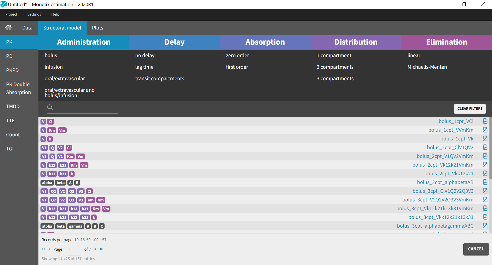
| The PK library is a library of standard PK models. Instead of writing the structural model yourself, you can select among simple PK models already written for you. When you select the PK library, a full list of all available models appear, which you can filter by selecting options for administration, distribution and elimination.
Here we provide general guidelines to guide you towards the standard PK model that is the most suited to your dataset. The guidelines are also summarized in this guidelines pdf. If you open any of the .txt files in this library, corresponding to the model written in mlxtran-formatted code, you see that the pkmodel macro is always used. This macro enables to define all standard PK models in a compact manner (except for multiple administration routes). It uses the analytical solution of the ODE system to simulate it, if it is available (which is the case for all models with linear elimination and without transit compartments), and otherwise the ODE system itself. A complete list of the analytical solutions for standard PK and PKPD models is available in this document. If none of the standard PK models seems to fit your needs, consider using a model from our other PK libraries (PK double absorption, TMDD). To define your own custom PK model, jump directly to data and models. |
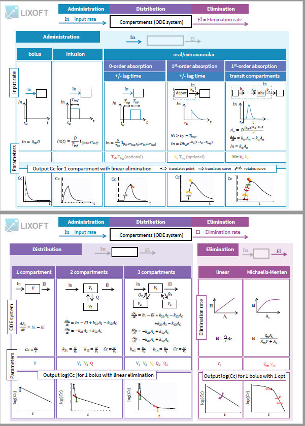
PK library cheat-sheet |
All PK models in the library correspond to a system of equations with the following structure:
- an input rate which depends on the type of administration
- an ODE system based on a number of compartments
- an elimination rate which depends on the type of elimination selected.
The equations express the concentration \( C_C(t)\) in the central compartment at a time t after the last drug administration:
- Single dose: at time \(t\) after dose D given at time
- Multiples doses: at time \(t\) after n doses
for i from \(1\) to \(n\) given at time
- Steady state: at a time \(t\) after dose \(D\) given at time
after repeated administration of dose \(D\) given at interval
(only for linear elimination)

 for i from \(1\) to \(n\) given at time
 (only for linear elimination)
Routes of administration
You should know the type of administration to use based on the study that generated the dataset. The route of administration will determine the dynamics of the input rate \(In(t)\) for the system described in Distribution.
To explore the differences in administration routes, we will see how they impact the input rate of a model with 1 compartment and linear elimination, parameterized with the clearance.

The ODE system for this model is:
\( \frac{d A_C}{dt} = In(t) – \frac{Cl}{V}A_C \)
\( C_C = \frac{A_C}{V} \)
Possible administration routes are![]()
![]()
![]()
![]()
Intravenous bolus
The intravenous bolus is an injection which quickly raises the concentration of the substance in the blood to an effective level. When bolus is selected, if \(D\) is the dose administered at time \(t_D\), we set the amount in the central compartment to \(A_C(t_D) = D\). This is equivalent to modeling the input rate as a dirac \(In(t) =\delta_{t_D}D \).
The response in the central compartment to a bolus in case of a model with 1 compartment with linear elimination is a decreasing exponential:

![]()
![]()
![]()
![]()
Infusion
This section focuses on intravenous infusion. For subcutaneous infusions, check the dedicated subsection in the oral/extravascular section.
To have the input modeled as an infusion instead of a bolus, you need to have a column tagged as ‘infusion rate’ or ‘infusion duration’ in your dataset in Monolix (the duration will be deduced from the amount and rate columns if rate is specified, and vice versa). In Simulx, you need to create a treatment element that is an infusion.
The intravenous infusion of duration \(T_{inf}\) sets the input rate to a constant value during the infusion, and then to zero: \(In(t) = \frac{D}{T_{inf}} \mathbf{1}_{[t_D, t_D + T_{inf}]}\).
The response in the central compartment in case of a model with 1 compartment with linear elimination is increasing as soon as the infusion starts, and decreasing as soon as it stops.
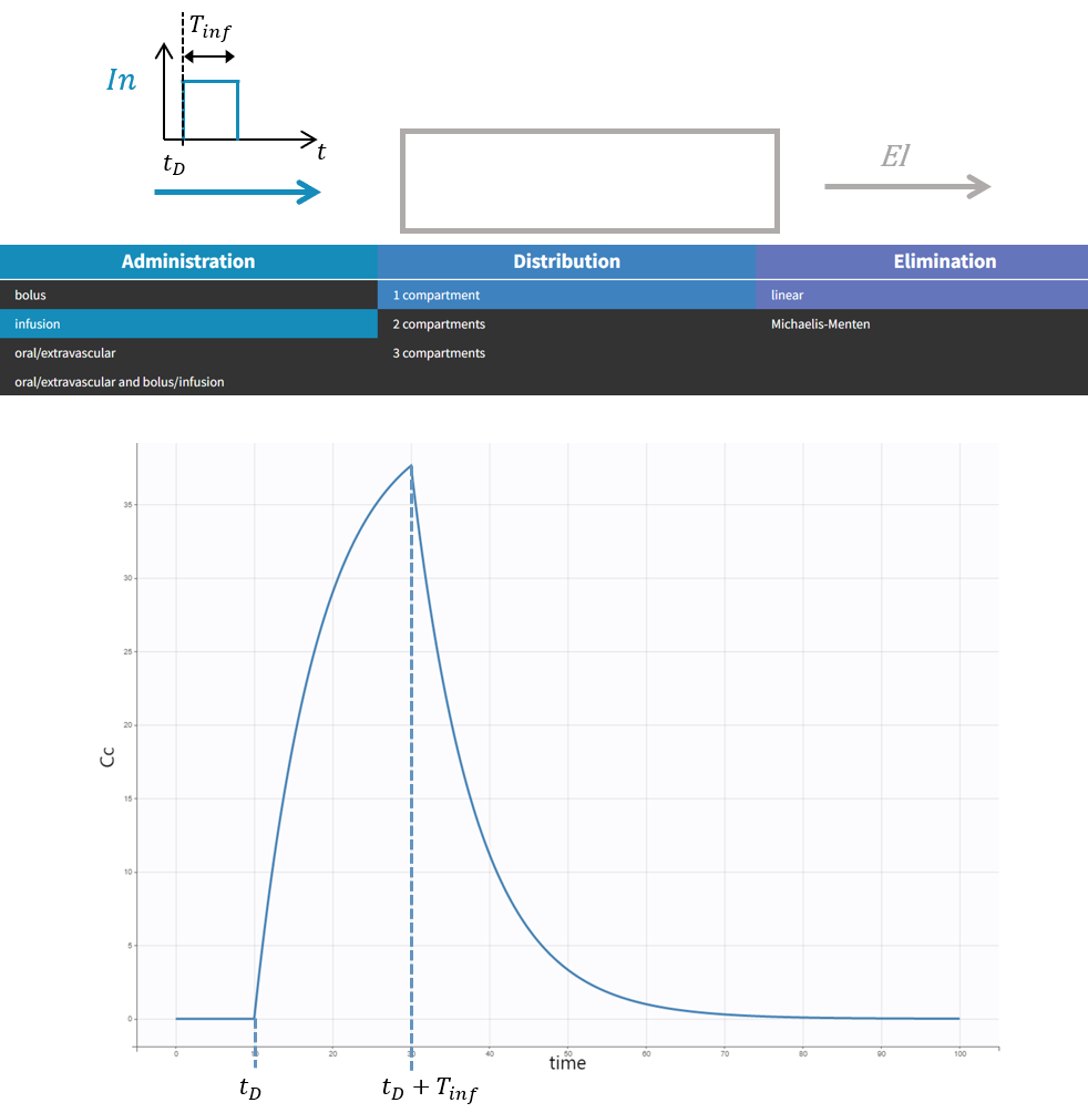
Note that bolus and infusion models are encoded exactly the same way with the pkmodel macro. It is the pkmodel macro that will check if a column tagged as INFUSION RATE or INFUSION DURATION appears in the dataset, and if this is the case, use the analytical solution of the infusion equations instead of the bolus equations.
Oral/extravascular administration
In the case of an oral or extravascular administration, you have additional options for delay and for the type of absorption.
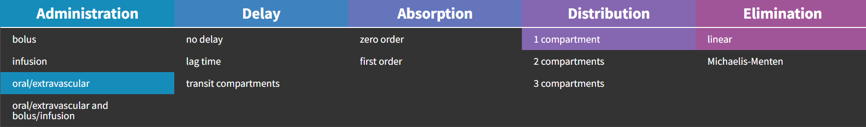
Absorption : 0 or 1st order?
The type of absorption will determine if the peak in the response is sharp or smooth.
A zero-order absorption is modeled with the same input rate as for an infusion, i.e. with a square pulse input, with 2 differences:
- the duration of the input \(T_{k0}\) is not known, it is thus part of the parameters to optimize, and it will influence the height and the duration of the response,
- a delay can be added between the dosing time and the start of the pulse, and this delay can also be optimized.
\(In^{0-order-lag}(t) = \frac{D}{T_{k0}} \mathbf{1}_{[t_D+T_{lag}, t_D+T_{lag} + T_{k0}]}\).
A first-order absorption will instead correspond to a sharper input pulse with a slow exponential decay which depends on the absorption rate. Because of this, the response peak is smoother. This input rate is the analytical solution of a system with a depot compartment where the dose would be added at time \(t_D+T_{lag}\), and which would be transferred to the central compartment with an absorption rate \(k_a\):
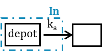
\(In^{1st-order-lag}(t) = D k_a e^{-k_a(t-t_D-T_{lag})} \mathbf{1}_{[t_D+T_{lag},\infty[}\).
We compare here zero and 1st order absorption in the case of a lag time, but if there is no lag in the response, the no delay option can be selected and the parameter \(T_{lag}\) will disappear.
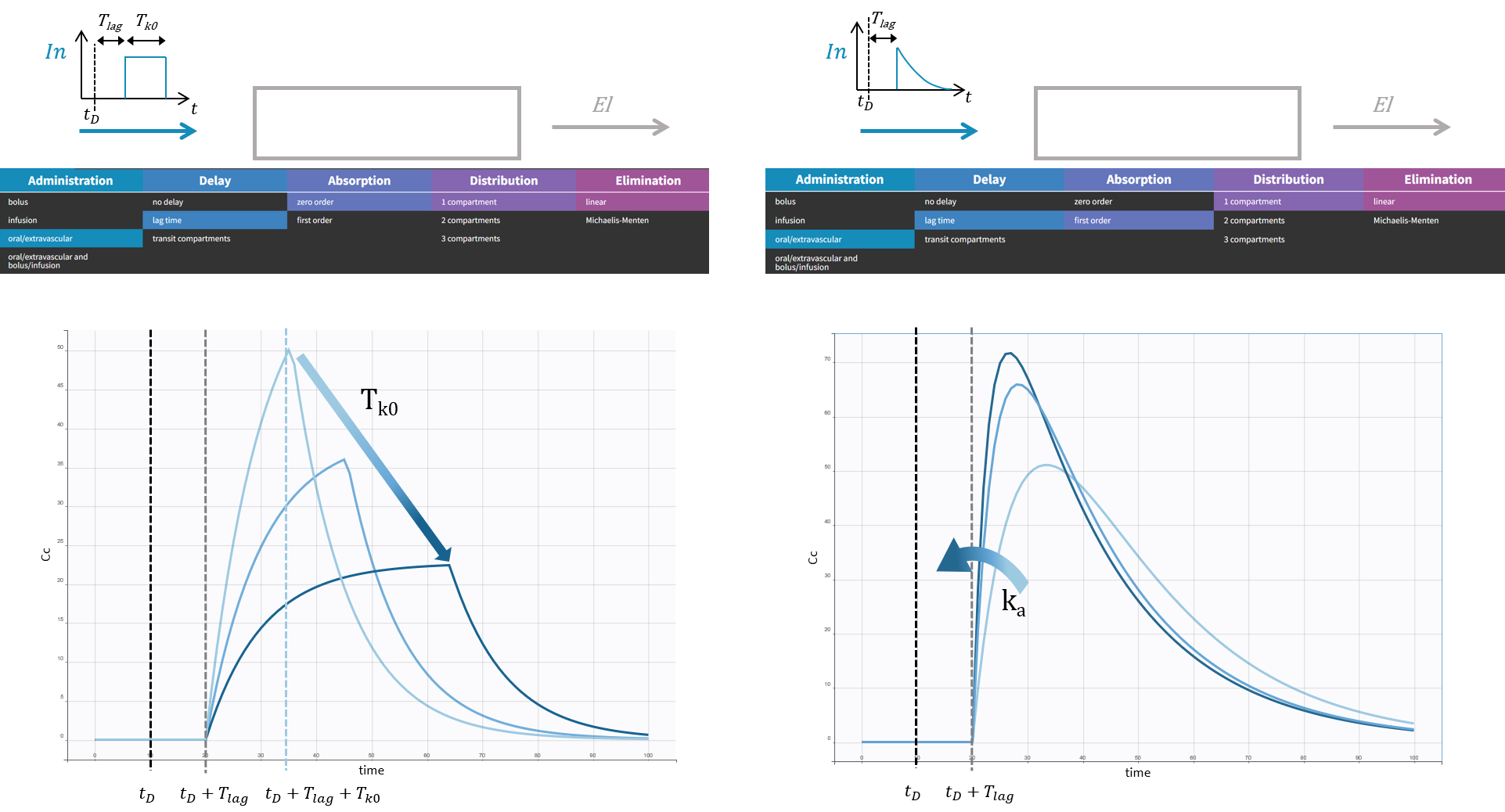
Delay: lag time or transit compartments?
In the case of a 1st order absorption, it is possible to select between two types of delay: a lag time or transit compartments. The type of delay selected will change the rising phase of the pulse input. A lag time corresponds to an instantaneous increase of the input rate at time \(t_D + T_{lag}\) whereas transit compartments will lead to a more gradual increase of the input rate right after \(t_D\). The rational for transit compartments and alternative phenomenological models for delayed absorption are described in a specific page. Transit compartments are sometimes more accurate than a lag time but the models take longer to simulate because there is no analytical solution available.
Instead of adding the dose to a depot compartment which would be also the absorption compartment at \(t_D+T_{lag}\), the dose is added at \(t_D\) but a number of transit compartments with transit rate \(k_{tr}\) between the compartments are added between the depot and the absorption compartment.
![]()
The input rate is the solution of the following system:
\(A_n = D\frac{(k_{tr}t)^ne^{-k_{tr}t}}{n!}\)
\(\frac{dA_a}{dt}=k_{tr}A_n-k_aA_a\)
\(In = k_a A_a\)
This absorption model gives more flexibility to fit the absorption phase with the 3 following parameters: transit rate \(k_{tr}\), the absorption rate \(k_a\) and the mean transit time \(M_{tt} = \frac{n+1}{k_{tr}}\).
![]()
Subcutaneous infusion
To have the input modeled as a subcutaneous infusion, you need to
- select a model with an oral/extravascular administration
- have a column tagged as ‘infusion rate’ or ‘infusion duration’ in your dataset in Monolix (the duration will be deduced from the amount and rate columns if rate is specified, and vice versa), or create a treatment element that is an infusion in Simulx.
Only 1st-order absorption is available in this case, and the input rate in case of Tlag (or no delay, i.e. Tlag = 0) is the solution of the following subsystem, combining the equations described above for infusion and for first-order absorption:
\(A_d (0) = 0\)
\(\frac{dA_d}{dt}=\frac{D}{T_{inf}}-k_a A_d\)
\(In (t) = k_a A_d (t-T_{lag})\)
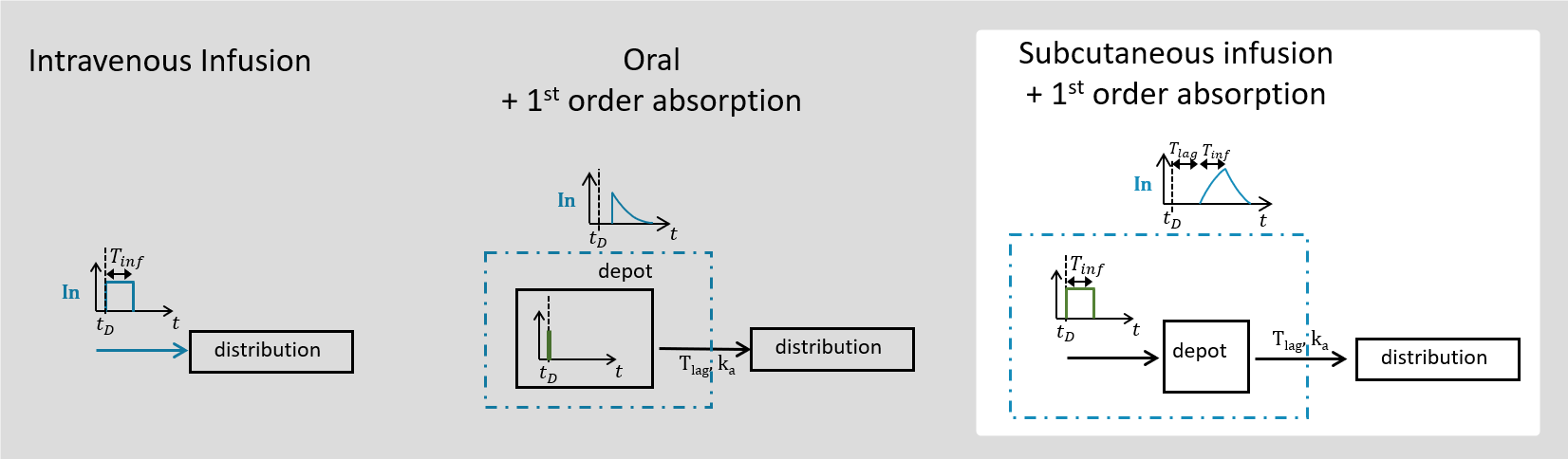
Multiple administration routes
It is possible to use a combination of an oral or extravascular administration, and a bolus or an infusion. For this, a column should be tagged as administration ID in the dataset with 1 for all doses administered intravenously and 2 for orally or extravascularly administered doses. In this case, the input rate is the sum of:
- an infusion rate if columns tagged as INFUSION RATE or INFUSION DURATION appear in the data, or a bolus rate otherwise,
- a rate for oral administration defined above.
For each of the combined models, there is a possibility to incorporate the bioavailability by selecting the model with parameter F. This will multiply the oral/extravascular administration input rate by the number F. We give this possibility only in case of multiple administration routes because in a single route setting, F and V would only appear in the ratio \(\frac{V}{F}\) which makes them non-identifiable.
Distribution
The input rate defined by the administration route impacts the amount of drug in the central compartment. You can select to have additional peripheral compartments leading to a system with 1, 2 or 3 compartments in total:
The ODE system for standard PK models involves one species per compartment. The amount of drug in the central compartment is called \(A_C\), and for the 2nd and 3rd compartment it is called \(A_2\) and \(A_3\). The output of the model is the concentration in the central compartment \(Cc\).
The ODE system for each case is given here, parameterized by the volumes in each compartment \(V_1, V_2, V_3\) and the intercompartmental clearance Q.

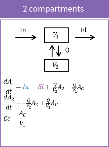
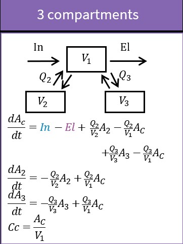
Instead of using the intercompartmental clearance \(Q_i\) between the central compartment and a peripheral compartment \(i\), and a volume \(V_i\) for each compartment, it is also possible to use the volume \(V\) in the central compartment only and transfer rates for each peripheral compartmental compartment \(i\): \(k_{1i} = \frac{Q_i}{V_1}, k_{i1} = \frac{Q_i}{V_i}\).
\(In\) and \(El\) rates are defined by the selected administration route and the elimination rate.
To show the impact of the number of compartments, we will see how they impact the response of a model with a bolus and linear elimination, parameterized with the clearance.

Impact of parameters in the case of 1 compartment
In the case of 1 compartment, the ODE system for a bolus with linear elimination parameterized with the clearance for \(t \ge t_D\) is:
\( A_C(t_D) = D\)
\( \frac{d A_C}{dt} = – \frac{Cl}{V}A_C \)
\( C_C = \frac{A_C}{V} \)
The response is given by a decreasing exponential \(\log(Cc) = \log(\frac{D}{V})-\frac{Cl}{V}(t-t_D)\). If the elimination rate \(\frac{Cl}{V}\) is kept constant (to focus on the effect of the distribution parameters), increasing the volume V will translate the whole response down:
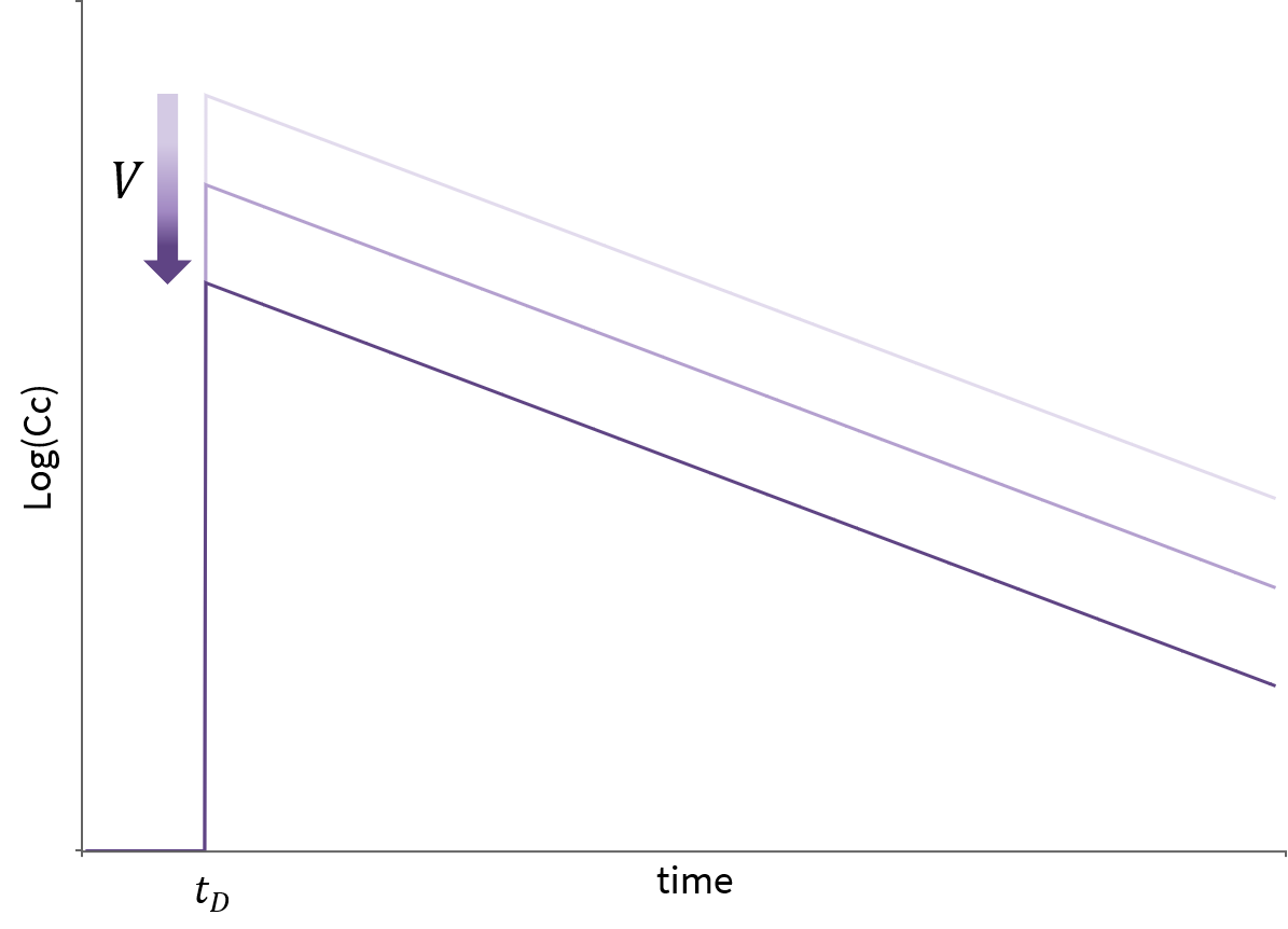
![]()
![]()
![]()
![]()
Impact of parameters in the case of 2 compartments
In the case of 2 compartments, the ODE system for a bolus with linear elimination leads to a response involving a sum of decreasing exponentials such that \(\log(Cc)\) shows 2 different slopes. Increasing \(V_1\) makes the response start lower, increasing \(V_2\) decreases the value at which the slope changes, and increasing \(Q\) moves this point earlier, making the slope change also sharper.
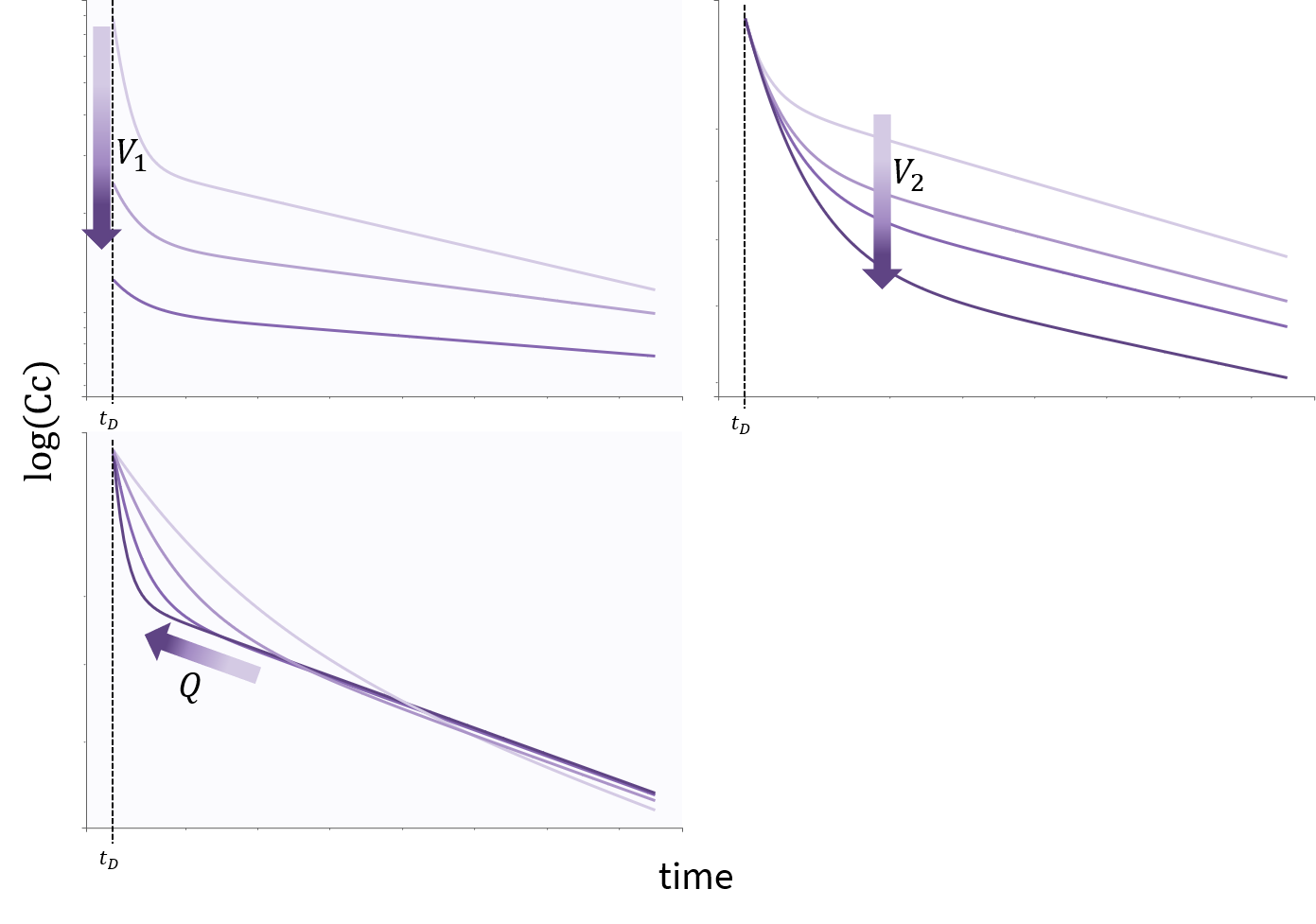
Impact of parameters in the case of 3 compartments
The case of 3 compartments is similar to the case of 2 compartments. \(\log(Cc)\) shows 3 different slopes. \(V_1\), \(V_2\) and \(Q_2\) influence the early dynamics by playing on the initial value, and on the time and height of the first point of slope change. \(Q_3\) and \(V_3\) influence the later dynamics by playing on the second point of slope change.
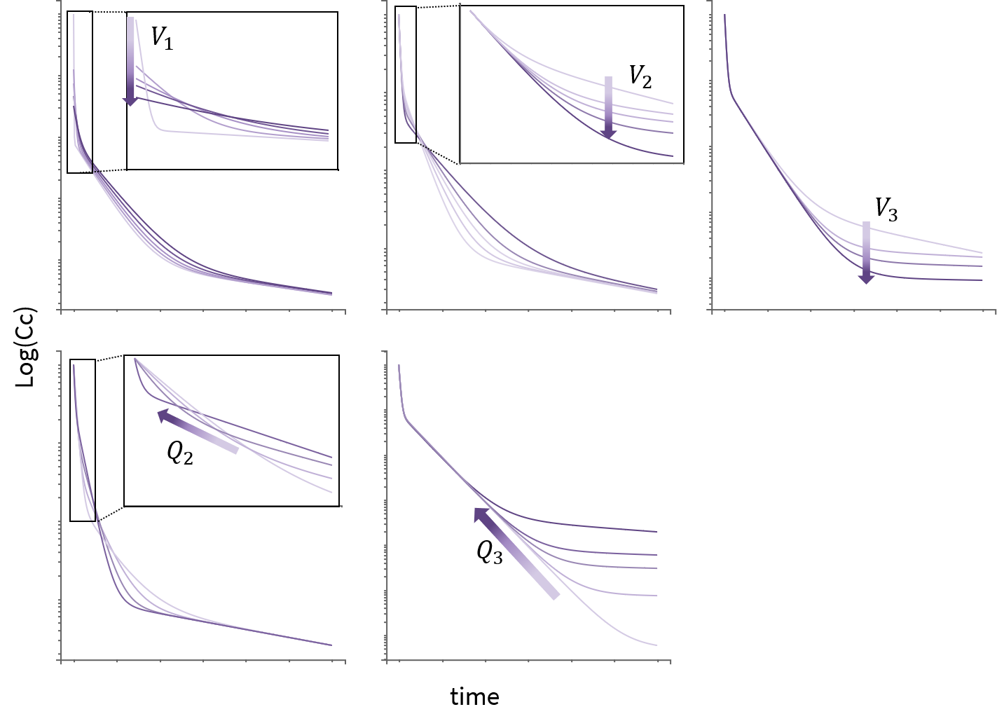
Elimination
The elimination rate denoted in the previous section as \(El\) can be either a linear rate involving the clearance \(Cl\), or a Michaelis Menten rate involving the constants \(K_m\) and \(V_m\). Another possible parameterization for the linear rate is using the elimination rate \(k = \frac{Cl}{V}\). To visualize the difference in the response, we show below the response of a 1-compartment model to a bolus in the two cases.
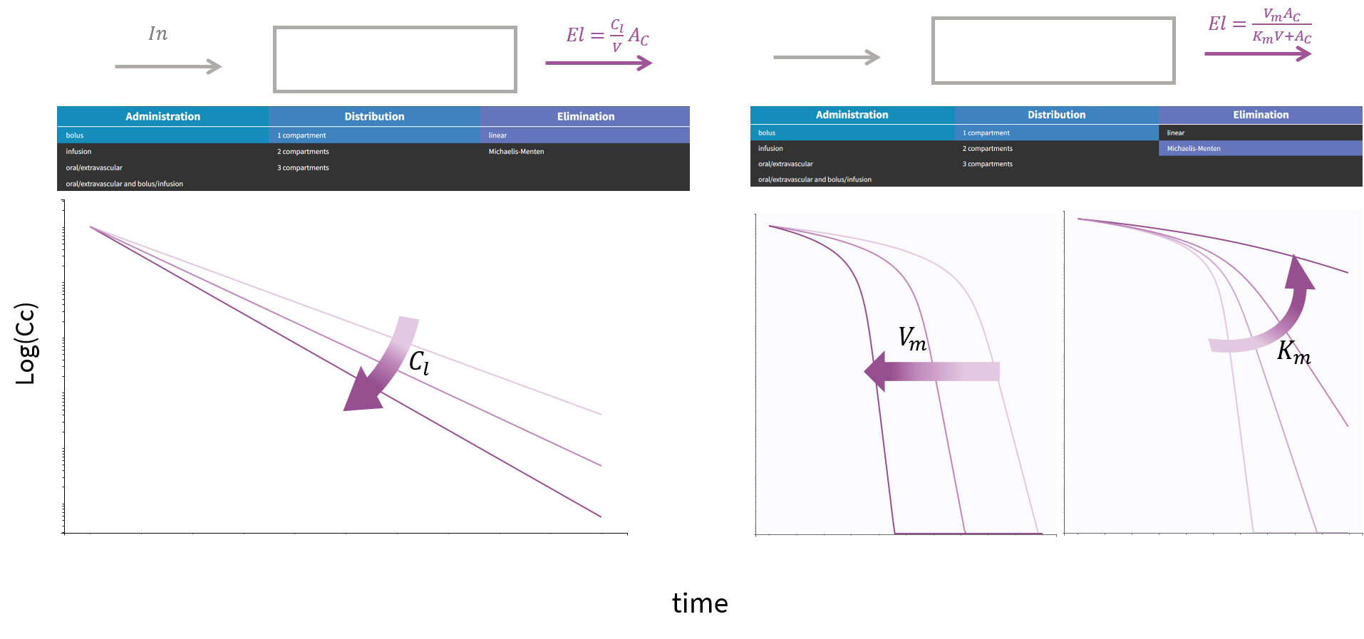
8.2.Library of PK models with double absorption
Some drugs can display complex absorption kinetics. Common examples are mixed first-order and zero-order absorptions, either sequentially or simultaneously, and fast and slow parallel first-order absorptions. Multiple peaks in concentration-time curves can also be described with mixed absorptions, and can be explained by different physiological processes, such as enterohepatic recycling, delayed gastric emptying, or variability of absorption.
In most cases, a two mixed absorptions are sufficient to capture the main features of the absorption.
We have developed a library of double absorption models implemented in Monolix to take into account all the combinations of absorption types and delays. The absorptions can be specified as simultaneous or sequential, and with a pre-defined or independent order. This library simplifies the selection and testing of different types of absorptions and delays.
Modeling choices
In this documentation we detail the filtering options in the interface of Monolix, shown on the figure below, and the corresponding parameters and modelling choices.
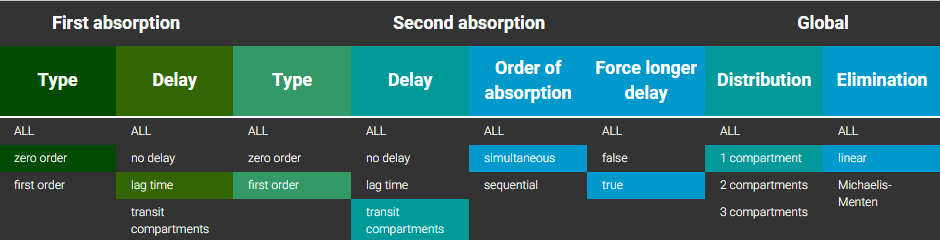
In all cases, a fraction F1 of the dose is absorbed via the first absorption and the remaining 1-F1 fraction of the dose is absorbed via the second absorption. As the parameter F1 must stay within [0,1], a logit distribution is automatically chosen, and the default initial value is 0.5.
The choices for the first absorption are:
- Type of absorption:
- zero order, modelled with the parameter Tk01
- first order, modelled with the parameter ka1
- Delay:
- no delay,
- a lag time, modelled with the parameter Tlag1
- transit compartments, modelled with the parameters Mtt1 (mean transit time) and Ktr1 (transfer rate)
The choices for the second absorption are:
- Type of absorption:
- zero order, modelled with the parameter Tk02
- first order, modelled with the parameter ka2
- Delay:
- no delay,
- a lag time, modelled with the parameter Tlag2
- transit compartments, modelled with the parameters Mtt2 (mean transit time) and Ktr2 (transfer rate)
- Order of absorption: this option is available if the first absorption is a zero-order type, otherwise absorptions are always simultaneous.
- Simultaneous: both absorptions are modelled with independent parameters. Depending on the values estimated for the parameters, the absorptions will be simultaneous or not.
- Sequential: the second absorption starts at the end of or after the zero-order process corresponding to the first absorption. So the second absorption is necessarily modelled with a delay, with two possible parameterizations:
- Tlag2 = Tk01 if “no delay” was chosen for both absorptions: the delay of the second absorption is equal to the duration of the first absorption.
- Tlag2 = Tlag1 + Tk01, if “lag time” was chosen for the first absorption and “no delay” was chosen for the second absorption.
- Tlag2 = Tk01 + diffTlag2, if “no delay” was chosen for the first absorption and “lag time” was chosen for the second absorption. In that case diffTlag2 is estimated instead of Tlag2, but the value of Tlag2 will be available in the outputs of Monolix thanks to the table statement. This parameterization ensures that the delay for the second absorption is greater than the duration of the first absorption.
- Tlag2 = Tlag1 + Tk01 + diffTlag2, if “lag time” was chosen for both absorptions. Similarly as before, diffTlag2 is estimated instead of Tlag2.
- Mtt2 = Tk01 + diffMtt2, if “no delay” was chosen for the first absorption and “transit compartments” was chosen for the second absorption. Similarly as before, diffMtt2 is estimated instead of Mtt2.
- Mtt2 = Tlag1 + Tk01 + diffMtt2, if “lag time” was chosen for the first absorption and “transit compartments” was chosen for the second absorption. Similarly as before, diffMtt2 is estimated instead of Mtt2.
- Force longer delay: this option is available if both absorptions where selected with a delay (lag time or transit compartments), and if the absorptions are not sequential.
- False: the parameters used to describe both delays are independent, so for the second absorption Tlag2 is estimated if “lag time” was chosen, and Mtt2 is estimated if “transit compartments” was chosen.
- True: similarly as above, the parameter for the delay of the second absorption is forced to be larger than the delay of the first absorption. For example, if “lag time” was chosen for both absorptions, Tlag2 is written as Tlag2 = Tlag1 + diffTlag2, and diffTlag2 is estimated instead of Tlag2.
Finally, just like for the PK library, the remaining choices are:
- Distribution:
- 1 compartment: the volume of the central compartment is V
- 2 compartments: the two compartments are modelled with the parameters V1 (volume of central compartment), Q (inter-compartment clearance) and V2 (volume of peripheral compartment), or with V (volume of central compartment), k12 and k21 (transfer rates between the central and peripheral compartments).
- 3 compartments: in the same way, the three compartments are modelled with V1, Q2, V2, Q3 and V3, or with V, k12, k21, k13 and k31.
- Elimination:
- Linear: modelled with Cl (clearance) or k (elimination rate)
- Michaelis-Menten: modelled with Vm and Km.
File names
The PK double absorption library contains many models, because of the many combinations of absorption types and delays for both absorptions, constraint on the time of the second absorption, distribution and parameterizations. In total 418 model files are available. The file names follow the pattern below:

In this pattern, oral0 means zero-order absorption, oral1 means first-order absorption, seqAbs corresponds to the filtering option “Order of absorptions = sequential” (the second absorptions starts at the end of the first absorption), and seqDelay corresponds to the filtering option “Force longer delay = true” (the delay for the second absorption is necessarily longer than the delay for the first absorption). If no keyword “seqDelay” or “seqAbs” are present in the file name, this is equivalent to the filtering option “Order of absorptions = sequential” and it means that the parameters for both absorptions are independent.
Examples
The models are written with PK macros.
For example, the model corresponding to a zero-order process with a lag time for the first absorption and a simulatenous (independent) first-order process with transit compartments for the second absorption, with a longer delay than the delay of the first absorption, a single compartment and parameterized with the clearance, is named oral0_oral1_seqDelay_1cpt_Tk01ka2F1Tlag1diffMtt2Ktr2VCl.txt and reads:
[LONGITUDINAL]
input = {Tk01, ka2, F1, Tlag1, diffMtt2, Ktr2, V, Cl}

EQUATION:
odeType=stiff

; Parameter transformations
k = Cl/V
Mtt2 = Tlag1 + diffMtt2

PK:
;PK model definition
compartment(cmt = 1, volume = V, concentration = Cc)
absorption(cmt = 1, Tk0 = Tk01, Tlag = Tlag1, p = F1)
absorption(cmt = 1, ka = ka2, Mtt = Mtt2, Ktr = Ktr2, p = 1-F1)
elimination(cmt = 1, k)

OUTPUT:
output = Cc
table = Mtt2
Other examples are available on this page.
Case study
A case study presenting a step-by-step modeling workflow for the PK of veralipride, using models from the double absorption library is available.
Veralipride plasma concentrations exhibit double peaks after oral absorption, due to site-specific absorption.
8.3.PK/PD model library
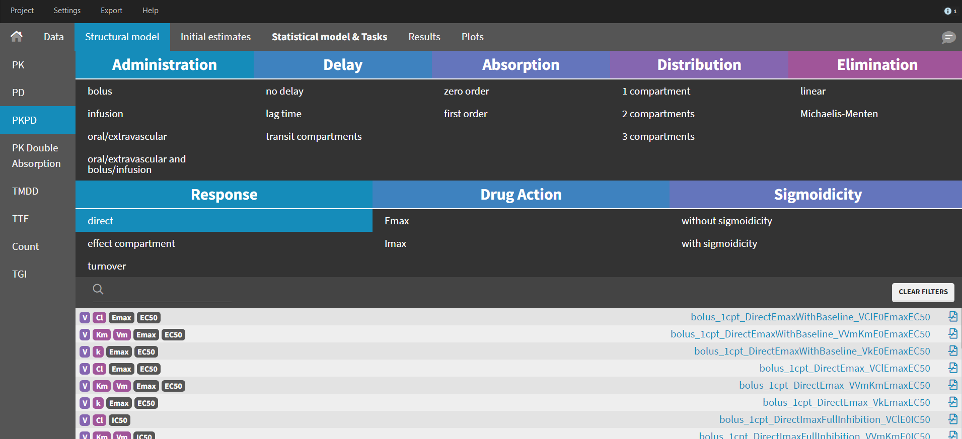
|
The PK/PD model library is combining our library of standard pharmacokinetic models with a library of standard pharmacodynamic models. The PK part is already described on the PK library page. Most PD models included in the PK/PD library can also be used alone (without a PK model) in the PD library, and some models from the PD library are only available alone. Here we provide general guidelines to guide you towards the standard PD model that is the most suited to your dataset. The guidelines are also summarized in this guidelines pdf.The complete list and full equations for PD models in the PD library is available in this document. Here we focus on the PD models of the PK/PD library because they are the most widely used. |
Cheat-sheet for the PD partof the PK/PD library |
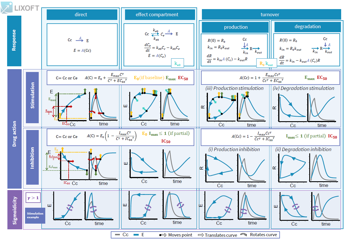
PD models can be categorized by:
- the type of response linking the concentration of the drug in the central compartment \(C_C\) to the effect E or to the response R. The effect can be either direct, or with an effect compartment, or an action on a turnover rate;
- the type of drug action on the response or on the rate. It can be a stimulation or an inhibition;
- the presence or absence of sigmoidicity in this drug action.
![]()
![]()
![]()
Type of response
The response links the drug concentration \(C_C\) to the effect \(E\) or the response R via a function \(A\) modeling the action of the drug. The type of response specifies whether this action impacts directly the effect, or via an effect compartment or turnover rates. The content of the action function will be specified in the next section: type of drug action. To explore the differences in the types of response, we will see how they impact the PD output for a 1 compartment PK linear infusion model, with a stimulation action of the drug and without sigmoidicity.
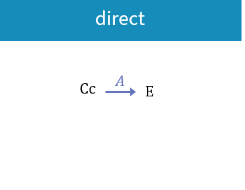
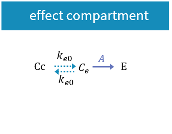

Direct
In case of a direct response, the effect \(E\) directly relates to the concentration in the central compartment \(C_C\) via
\(E = A(C_C)\)
Therefore the dynamics of the effect follow the dynamics of \(C_C\) without any delay, meaning that as soon as \(C_C\) starts decreasing, \(E\) decreases as well, and the trajectory in the phase plane \(C_C\) vs \(E\) is a single line because it follows the same route during the increase and the decrease of the signals. Below is an example simulation of a direct model with a stimulation action of the drug on the PD.
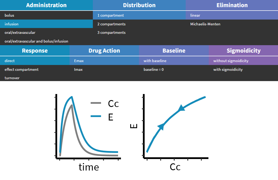
Effect compartment
The site of action of the drug is often not be the same as the central compartment, and therefore a delay often appears between the PK and the PD measurements. To account for this delay it may be enough to add a single theoretical effect compartment with a drug concentration \(C_e\) equal to the concentration at the site of action. This theoretical compartment is assumed not to impact the concentration in the central compartment \(C_C\), therefore we write the transfer arrows between the central compartment and the effect compartment with dashed lines. A single transfer rate \(k_{e0}\) is used and the effect now directly relates to \(C_e\):
\(\frac{d C_e}{dt} = k_{e0}C_C – k_{e0}C_e\)
\(E = A(C_e)\)
Below is an example simulation of a model with an effect compartment and with a stimulation action of the drug on the PD. The higher the transfer parameter ke0, the higher the response and shorter the delay in the response.
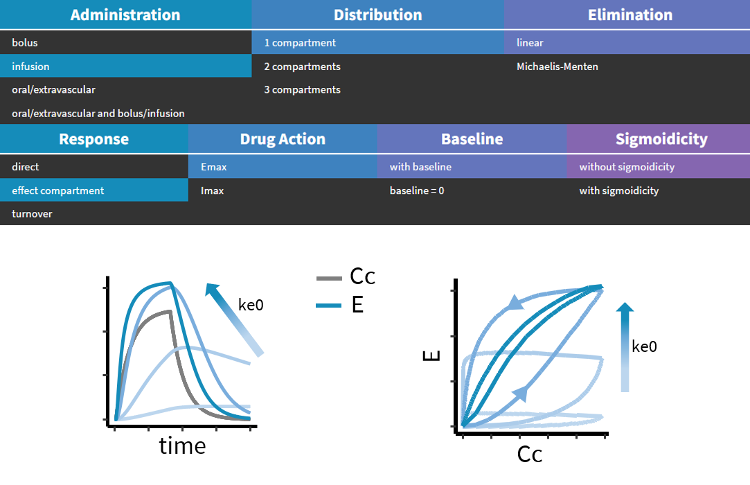
Turnover
To model a PD response showing delay compared to the PK, it is also possible to consider that the PK concentration has an impact on the production or the degradation rate of a response variable R, as described by Sharma et al (1998). The response is then modeled with the following ODE:
- if action on the production rate: \(\frac{d R}{dt} = k_{in}A(C_C) – k_{out}R\)
- if action on the degradation rate: \(\frac{d R}{dt} = k_{in} – k_{out}A(C_C)R\)
In both cases, the model can be parameterized with the initial value of R \(R_0\) and the parameter \(k_{out}\), and \(k_{in}\) is derived as \(k_{in} = R_0 k_{out}\).
We compare below the response in the case of production stimulation and degradation inhibition. \(k_{out}\) plays a similar role as \(ke0\) in the case of an effect compartment: the higer \(k_{out}\), the shorter the delay.
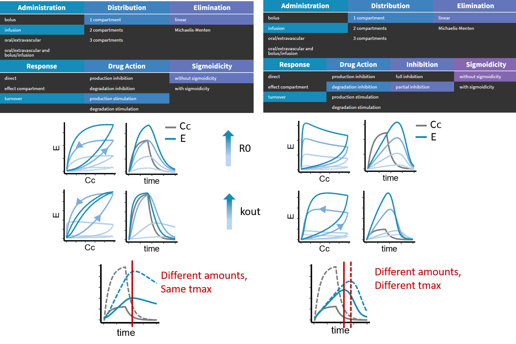
The difference between a turnover effect on the production or on the degradation is not obvious when checking the response to a single dose amount. A clear difference can be seen if two different dose amounts are given to the same individual. In the case of a turnover on production, the responses will show exactly the same delay, whereas in the case of a turnover on degradation, the delay in the response will be different for different dose amounts.
Type of drug action
The type of drug action will determine the function A relating the PK concentration to the PD effect. It can be a stimulation or an inhibition, and it is written differently depending on the type of response.
Stimulation
- In the case of a direct model or an effect compartment, the action of stimulation is parameterized with \(E_{max}\), \(EC_{50}\), \(\gamma\) if sigmoidicity is selected (otherwise \(\gamma = 1\)), and \(E_0\) if baseline is selected (otherwise \(E_0 = 0\)). The equation for A in the most general case is:
\(A(C) = E_0 + \frac{E_{max}C^{\gamma}}{C^{\gamma} + EC_{50}^\gamma}\)
where C is the concentration in the central compartment \(C_C\) if the model is direct, and the concentration in the effect compartment \(C_E\) if the model includes an effect compartment.
- In the case of a turnover model, the action of stimulation can happen on the production or on the degradation rate. In any case, it is parameterized with \(E_{max}\), \(EC_{50}\), and \(\gamma\) if sigmoidicity is selected, and the function always takes as an input the concentration in the central compartment \(C_C\). \(E_0\) does not appear because turnover models already include a parameter \(R_0\) to model the initial value of the response R.
\(A(C_C) = 1 + \frac{E_{max}C_C^{\gamma}}{C_C^{\gamma} + EC_{50}^\gamma}\)
Below is the example response of a direct model with a stimulation action (called Emax in the drug action section of the library) and without sigmoidicity (\(\gamma = 1\)). We show the influence of increasing E0, Emax, or the EC50. The influence of the sigmoidicity parameter \(\gamma\) is shown in the next section.
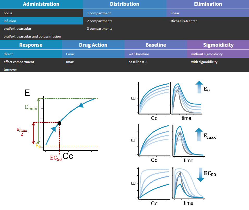
Inhibition
- In the case of a direct model or an effect compartment, the action of inhibition is parameterized with \(E_0\), \(IC_{50}\), \(I_{max}\) if partial inhibition is selected (otherwise \(I_{max} = 1\)), \(\gamma\) if sigmoidicity is selected (otherwise \(\gamma = 1\)). The equation for A in the most general case is:
\(A(C) = E_0 \Big( 1 – \frac{I_{max}C^{\gamma}}{C^{\gamma} + EC_{50}^\gamma} \Big) \)
where C is the concentration in the central compartment \(C_C\) if the model is direct, and the concentration in the effect compartment \(C_E\) if the model includes an effect compartment.
- In the case of a turnover model, the action of inhibition can happen on the production or on the degradation rate. In any case, it is parameterized with\(IC_{50}\), \(I_{max}\) if partial inhibition is selected (otherwise \(I_{max} = 1\)), and \(\gamma\) if sigmoidicity is selected, and the function always takes as an input the concentration in the central compartment \(C_C\). \(E_0\) does not appear because turnover models already include a parameter \(R_0\) to model the initial value of the response R.
\(A(C_C) = 1 – \frac{I_{max}C_C^{\gamma}}{C_C^{\gamma} + IC_{50}^\gamma}\)
Below is the example response of a direct model with an inhibition type of action (called Imax in the drug action section of the library) and without sigmoidicity (\(\gamma = 1\)). We show the influence of increasing Imax, or the IC50. The influence of the sigmoidicity parameter \(\gamma\) is shown in the next section.
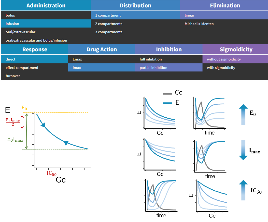
Sigmoidicity
Whether it is a stimulation or an inhibition type of action, the drug action function can always involve an exponent parameter \(\gamma\). If this parameter is higher than 1, the response curve in the phase plane (\(C_C\) vs \(E\)) looks more like a sigmoid. Sigmoidicity can impact the dynamics in the PD response, making the response more switch-like due to threshold effects. If sigmoidicity is selected, the parameter \(\gamma\) will be estimated.
Below is the example response of a direct model with a stimulation type of action, and with sigmoidicity. The higher the gamma, the steeper the dose response, and the more square-like the time response.
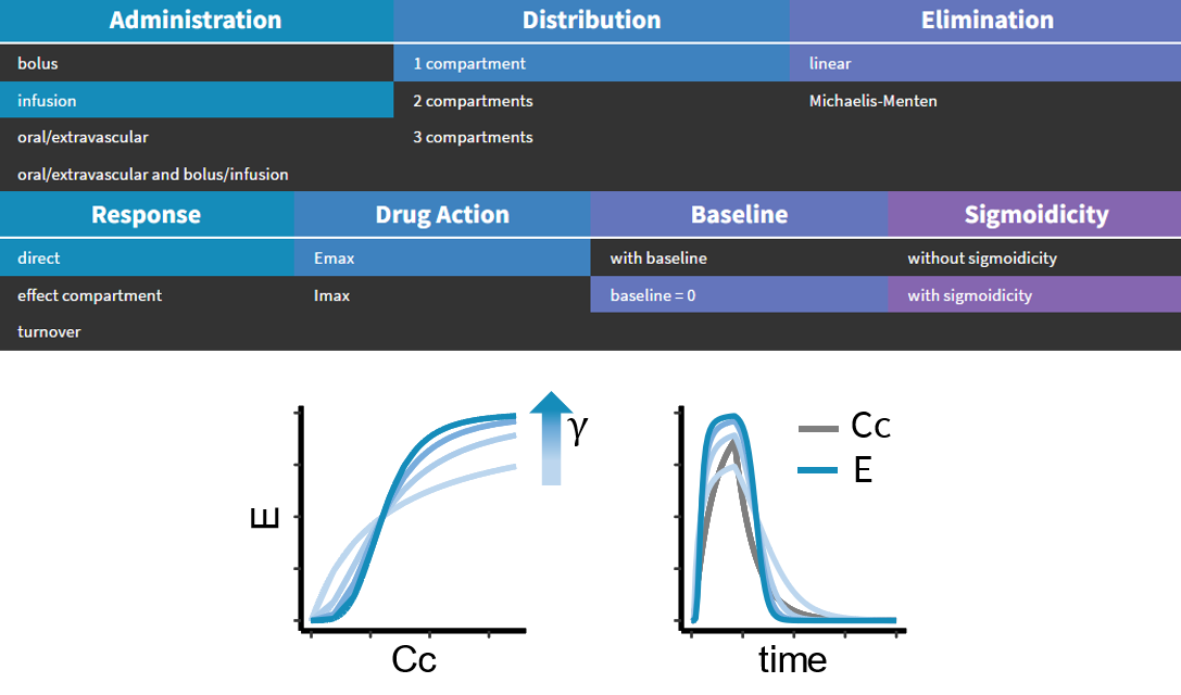
8.4.Library of Parent - Metabolite models
Drugs can undergo a transformation into metabolites – pharmacologically active and/or producing adverse effects. They can impact the pharmacokinetics of the parent and drive the efficacy. But, at the same time, can rise safety concerns. Joint parent – metabolite models account for the impact of the parent-metabolite interactions on the estimation.
Library of Parent – Metabolite models includes many characteristic mechanisms, such as first pass effect, uni and bidirectional transformation and up to three compartments for parent and metabolite, which makes it an excellent tool for exploration and modeling. Implementation with mlxtran macros uses analytical solutions for faster parameter estimation and makes a great basis for the development of more complex models.
AdministrationSelect administration route, delay, absorption mechanism and first pass effect to correctly model drug input. |
TransformationCheck non-reversible and reversible metabolic systems to predict the impact of parent-metabolite interactions. |
DistributionExplore different number of peripheral compartments independently for parent and metabolite. |
EliminationTry linear or non-linear Michaelis-Menten elimination mechanism to get a better fit. |
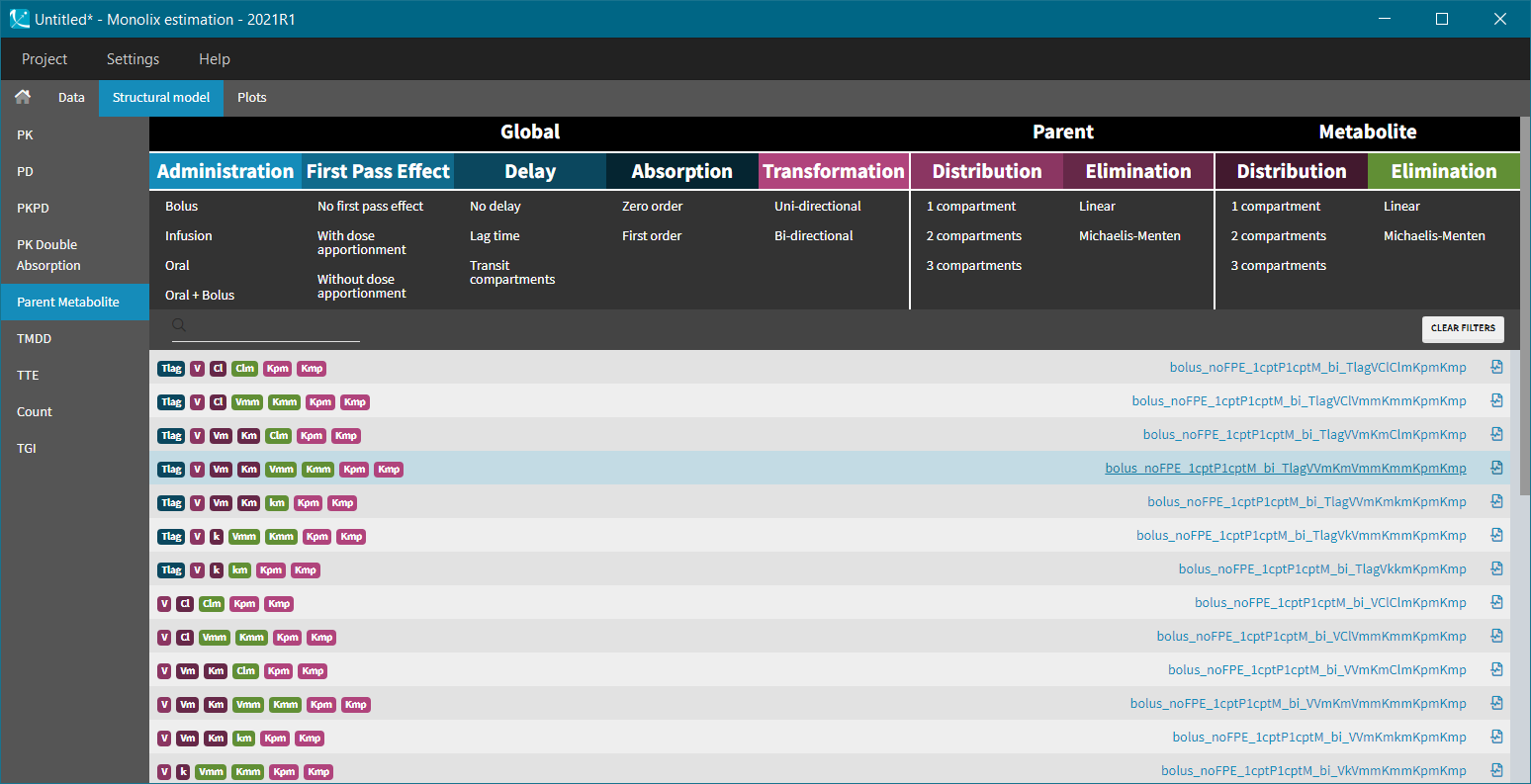
Parent-metabolite model filters
Administration
Parent-metabolite models can be combined with standard administration routes: bolus, infusion, oral/extravascular and oral with bolus. Intravenous doses are always administered to the central parent compartment. Oral doses can be in addition split between parent and metabolite – the first pass effect.
Intravenous doses (bolus, infusion) are always administered to the central parent compartment, can be with or without a time delay and does not include the first pass effect.
Oral doses can be with the following options:
- with or without the first pass effect
- zero (Tk0) or first order absorption process (ka for parent, kam for metabolite in case of the first pass effect)
- without or with a time delay (Tlag) or with the transit compartments (Mtt, Ktr)
- oral + bolus: bioavailability F (estimated as a separated parameter)
|
Without First Pass Effect |
With First Pass Effect |
|||||||||
 |
Without dose apportionment |
With dose apportionment |
||||||||
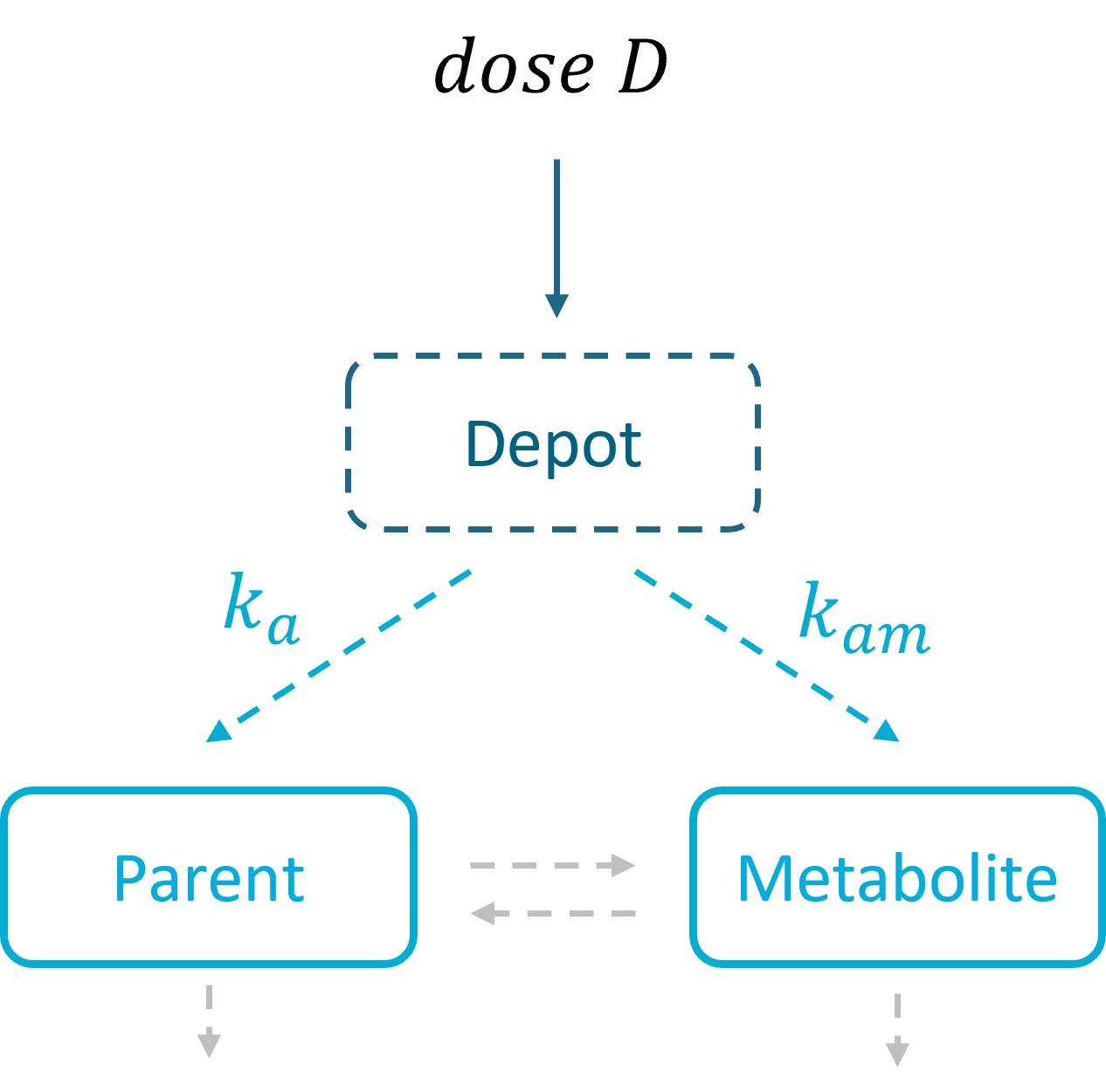 |
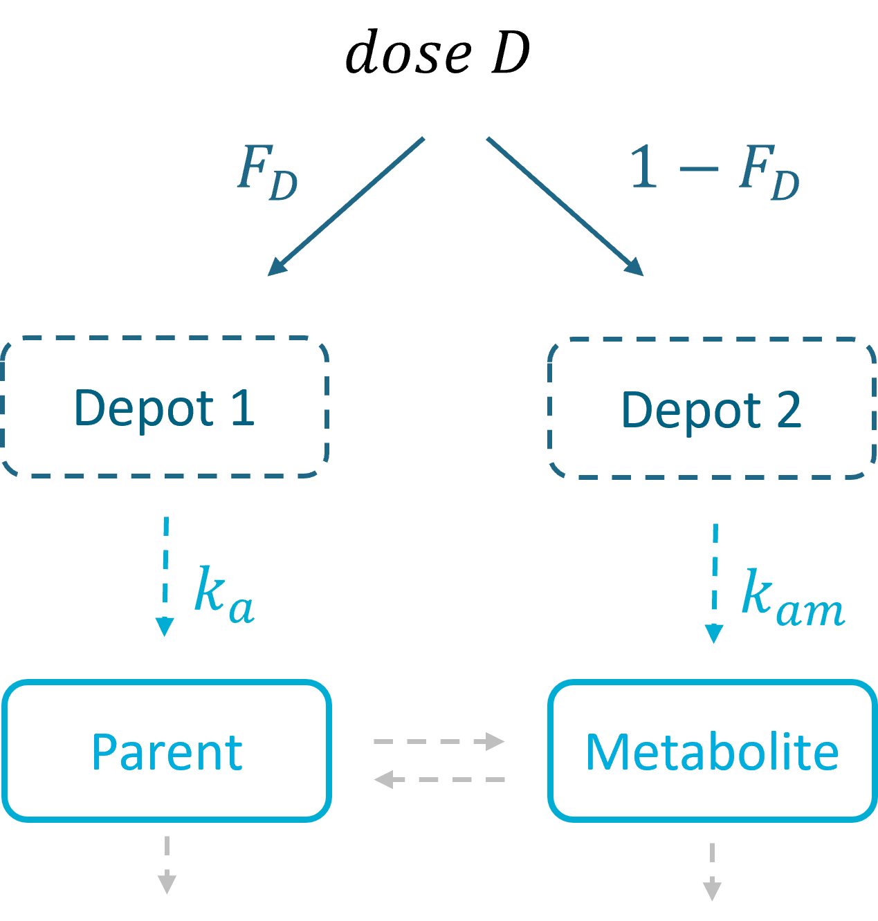 |
|||||||||
|
Oral first order:
Oral zero order: the same formulas, with Tk0, Tk0m in place of ka, kam |
Oral first order:
Oral zero order: the same formulas, with Tk0, Tk0m in place of ka, kam |
||||||||


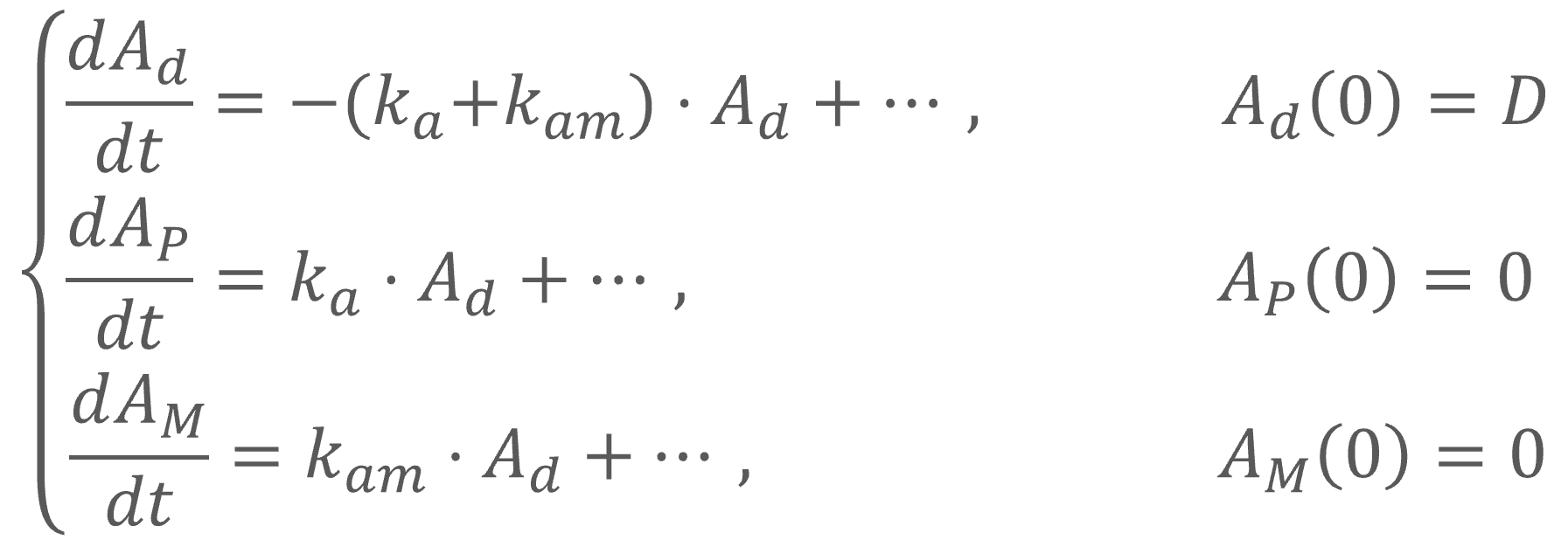

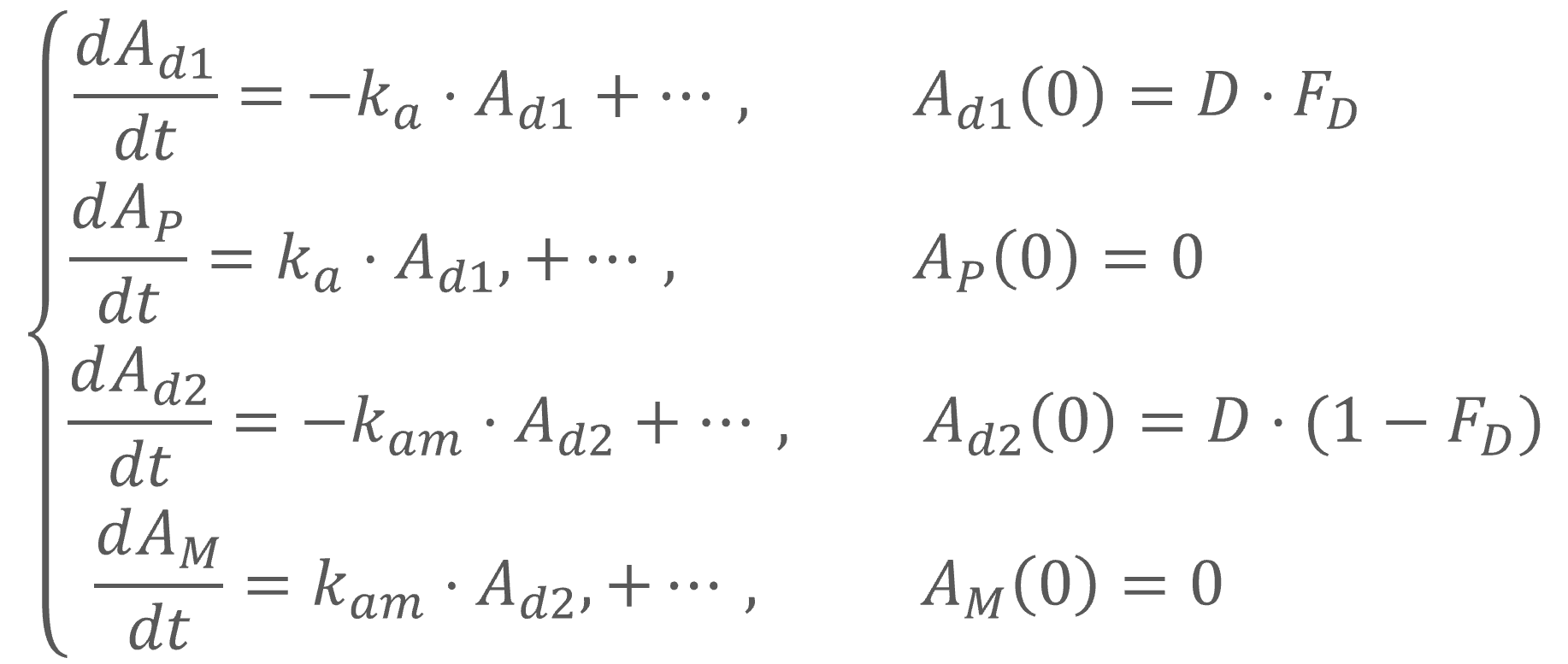

First pass effect
The first pass effect is a phenomenon in which a drug undergoes any biotransformation at a specific location in the body – for example transformation of parent to metabolite before reaching its site of action or the systemic circulation. The first-pass effect can be clinically relevant when the metabolized fraction is high or when it varies significantly from individual to individual or within the same individual over time, resulting in variable or erratic absorption. It also has an impact on peak drug concentrations, which may result in parent concentration peaks occurring much earlier.
In the Monolix library, models with the first pass effect include splitting a dose – with or without dose apportionment – and absorbing one fraction in the central parent compartment (Tk0 or ka) and the other fraction in the central metabolite compartment (Tk0m or kam). The absorption process, zero or first order, is the same for parent and metabolite.
- Dose apportionment means that the splitting is independent of the absorption constants (Tk0, Tk0m or ka, kam), with a fraction F_D of the dose leading to the parent and a fraction 1 – F_D leading to the metabolite prior to reach the plasma.
- In models without dose apportionment, dose splitting is implicit and results from different absorption rates ka, kam (or absorption times Tk0, Tk0m).
Distribution

In the library it is possible to select different number of compartments for parent and for metabolite. The central compartments have the same volume V – identifiability issue when only parent drug is administered.
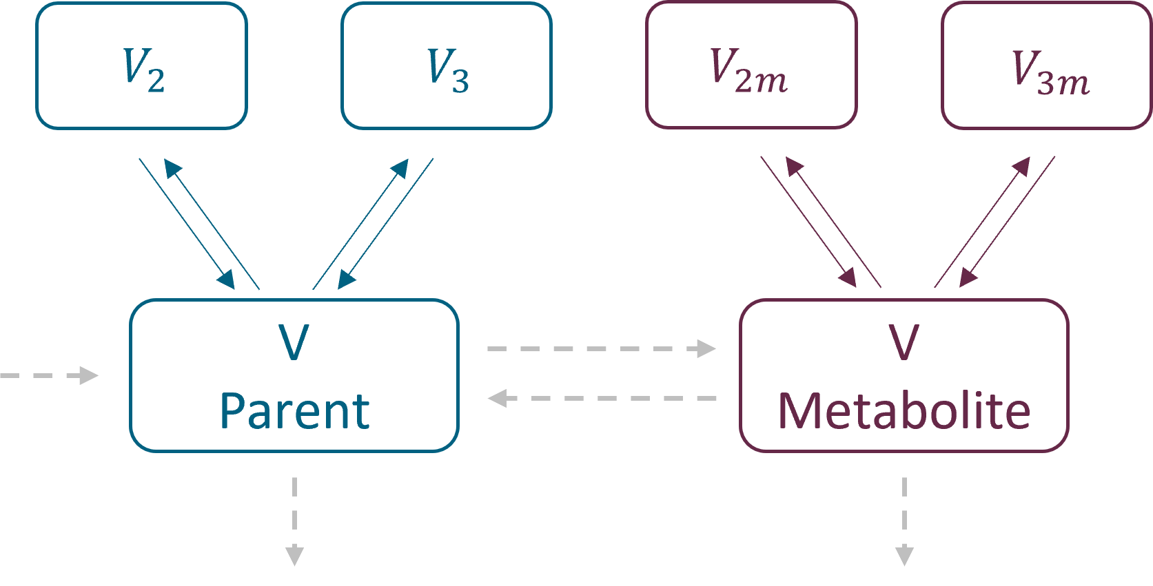
Parametrization
Parent and metabolite have the same parametrization. As for the PK and PKPD libraries, there are two parametrizations available:
- with exchange rates: k12, k21 for parent and k12m, k21m for metabolite for the second compartments, and k13, k31 and k13m, k31m for the third compartments. Peripheral compartments are defined implicitly through the exchange rates, so volumes V2, V3, V2m and V3m are not estimated. The volume of central compartments is V (for both parent and metabolite)
- with inter – compartment clearance: Q2, V2, Q3, V3 for parent and Q2m, V2m, Q3m, V3m for metabolite. The volume of central compartments is V1 (for both parent and metabolite), to be compatible with the PK models in case of the sequential model development.
Transformation and elimination
Drug, after administration is eliminated from the system or transformed into metabolite, which subsequently is also eliminated. In addition, metabolite can be back-transformed into a parent – it is a common process for example for amines. Both, unidirectional and reversible, transformations can be selected from the “global” section of filters in the Monolix parent-metabolite library. Elimination, linear or non-linear (Michaelis-Menten), is specific for parent and for metabolite.
- Transformation:
- Kpm – transformation rate from parent to metabolite
- Kmp – transformation rate from metabolite to parent
![]()
- Elimination: parent and metabolite can be eliminated with different process (linear or non-linear)
- Cl, k, Vm, Km – elimination parameters for parent
- Clm, km, Vmm, Kmm – elimination parameters for metabolite
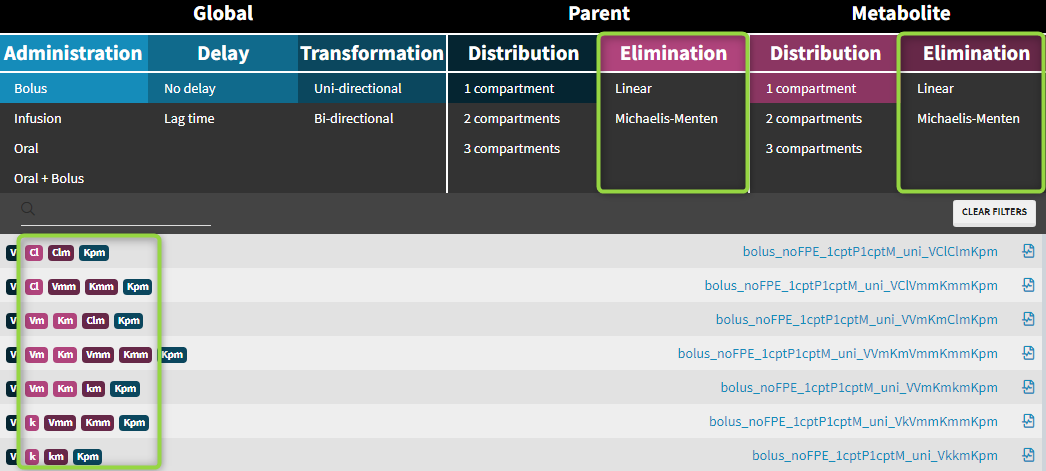
Examples:
![]()
Analytical solutions
Implementation in the Mlxtran
Example: a model with oral absorption (rate ka) of a dose D, one central compartment for parent (cmt = 1) and one for metabolite (cmt = 2), linear elimination (rates: k, km) and uni-directional transformation (rate Kpm), is the following:
where 


 = 0, C_{m}(0) = 0,")
Models in the parent-metabolite Monolix library are build using mlxtran macros. For the above model:
;PK model definition for parent
compartment(cmt = 1, volume = V, concentration = Cp)
oral(cmt = 1, ka)
elimination(cmt = 1, k)
;PK model definition for metabolite
compartment(cmt = 2, volume = V, concentration = Cm)
elimination(cmt = 2, k = km)
transfer(from = 1, to = 2, kt = Kpm)
Analytical solutions
Analytical solutions, which are more accurate than numerical solutions and are faster than ODE solvers, are implemented for parent – metabolite models satisfying the following conditions:
- administration (bolus, IV, oral 0 or 1st order) is to the central parent compartment only => models from the library with first pass effect (“with dose apportionment” and “without dose apportionment”) do not use analytical solutions
- parameters are not time dependent (exception: dose coefficients such as Tlag, which are evaluated only once),
- elimination is linear and only from the central parent and/or metabolite compartments, => models from the library with elimination = “Michaelis-Menten” do not use the analytical solutions
- there are no transit compartments, => models from the library with delay = “transit compartments” do not use the analytical solution
- transfer between parent and metabolite is only between their central compartments,
- there are maximally two peripheral compartments for parent and maximally two for metabolite.
Comparison of the performance between analytical and numerical solutions
The following example compares the computational time (in seconds) of the parameter estimation task (SAEM) using analytical solutions (AS) and numerical solutions (ODE) for models with different number of compartments.
Dataset: simulated in Simulx N = 100 individuals, who received a single or multi oral doses. 5 or 20 measurements of both, parent and metabolite concentrations registered for each individual.
SAEM: (fixed number of iterations) 500 iterations for the exploratory phase, 200 iterations for the smoothing phase.

Times are given in seconds, and values in bold give the speed up ratio when using an analytical solution.
8.5.Target-mediated drug disposition (TMDD) model library
This page presents the TMDD model library proposed by Lixoft. It includes an introduction to the TMDD concepts, the description of the library’s content, a detailed explanation of the hierarchy of TMDD model approximations, and guidelines to choose an appropriate model.
You can download the library here. All the models are text files. To use it, extract all in a TMDD folder for example.
- Introduction to TMDD concepts
- The TMDD model library
- Overview of the hierarchy of TMDD models and approximations
- Detailed description of TMDD approximations
- Guidelines to choose an appropriate model
- Typical parameters for TMDD
- Examples of molecules
- Extensions to more complex TMDD models
Introduction to TMDD concepts
The concept of TMDD has been proposed as an explanation to the non-linear behavior (violation of the superposition principle and dose-dependent volume of distribution) displayed by some drugs such as bosentan. The concept was first formulated by Gerhard Levy in
Levy describes the TMDD in the following way: “a considerably larger fraction of the dose of these high-affinity compounds is bound to target sites, enough so that this interaction is reflected in the pharmacokinetic characteristics of the drug.”
Target-mediated drug disposition happens when the binding of the drug to the target influences the drugs distribution and elimination. This is in particular often the case for biologics (see section Examples of molecules), such as monoclonal antibodies for instance (for a review, see for instance Dostalek et al. (2013)), because they are designed to be highly specific and strongly bind to their target. In this case, the drug is eliminated both via usual linear clearance mechanisms, that dominate at high concentrations when the target is saturated, and non-linear target-mediated clearance (via binding and internalization of the drug-target complex), that is mainly visible at low concentrations.
The interplay of these mechanisms results in complex concentration-time curves. To describe the observed data, Mager and Jusko ((2001) JPP 28(6)) have introduced a set of equations that includes:
- the linear elimination of the ligand (elimination rate kel)
- the turnover of the receptor (synthesis rate ksyn, degradation rate kdeg, initial receptor concentration R0=ksyn/kdeg)
- the binding of the ligand to the receptor to form the complex (binding rate kon, dissociation rate koff, dissociation constant KD=koff/kon)
- the internalization of the complex (rate kint)
- (optional) the distribution of the ligand to a peripheral compartment (rates k12 and k21)

A key characteristic of TMDD systems is that the pharmacokinetic behavior depends on the dose. Let us focus on the free ligand concentration-time course with several doses of different magnitudes. In the figure below, we look at the concentration (on log-scale) with respect to time. In addition, we use a bolus administration and a single compartment for the ligand (the two compartment case will be studied later on).
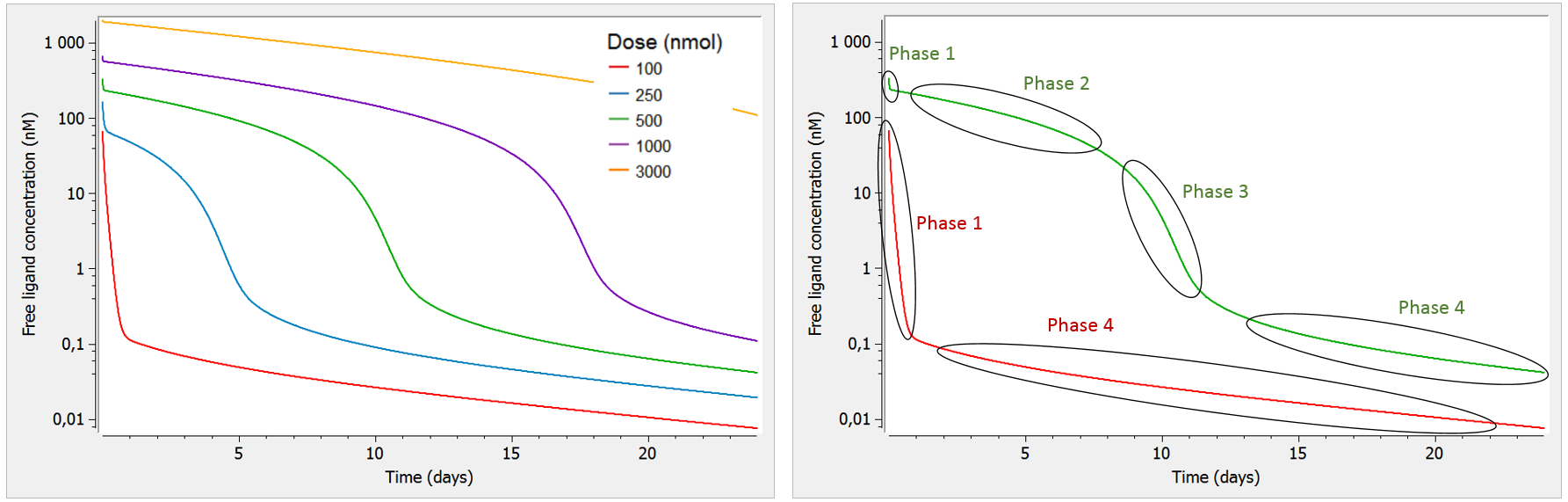
As can be seen on the green curve, when the initial concentration of ligand is larger than the initial receptor concentration (here R0=100), the ligand concentration-time curve displays a complex shape (see also Peletier et al. (2012)) with:
- Phase 1: steep initial decrease, corresponding to the rapid binding of the ligand to the receptor.
- Phase 2: linear elimination phase, where the receptor is saturated with ligands (almost no more binding of ligand to receptor happens), and the ligand is eliminated via usual elimination processes (renal filtration, etc).
- Phase 3: transition phase, where the ligand binds to the no-longer saturated receptor.
- Phase 4: terminal elimination phase, where elimination of the free ligand happens mainly due to internalization (or degradation) of the target/receptor, which shifts the binding equilibrium out of balance leading to new binding of ligand.
Note that we focus on the concentration of the free ligand, such that binding of the ligand to the receptor constitutes an “elimination” mechanism in that it reduces the concentration of free ligand.
On the opposite, as can be seen on the red curve, if the initial ligand concentration is of the same order of magnitude or lower than the receptor concentration (here R0=100), the free ligand concentration time-curve displays two phases:
- Phase 1: steep initial decrease, corresponding to the rapid binding of the ligand to the receptor
- Phase 4: terminal elimination phase, where elimination of the free ligand happens mainly due to internalization (or degradation) of the target/receptor, which shifts the binding equilibrium out of balance leading to new binding of ligand
Note that in this case, the receptor is never saturated with ligand and target-mediated elimination usually dominates over the linear elimination. Thus, the curve goes directly from phase 1 to phase 4.
Below we show the typical concentration-time curves for the other entities in linear scale and log scale. The total ligand Ltot is the sum of free ligand L and bound ligand P (complex). The total receptor Rtot is the sum of free receptor R and bound receptor P (complex).

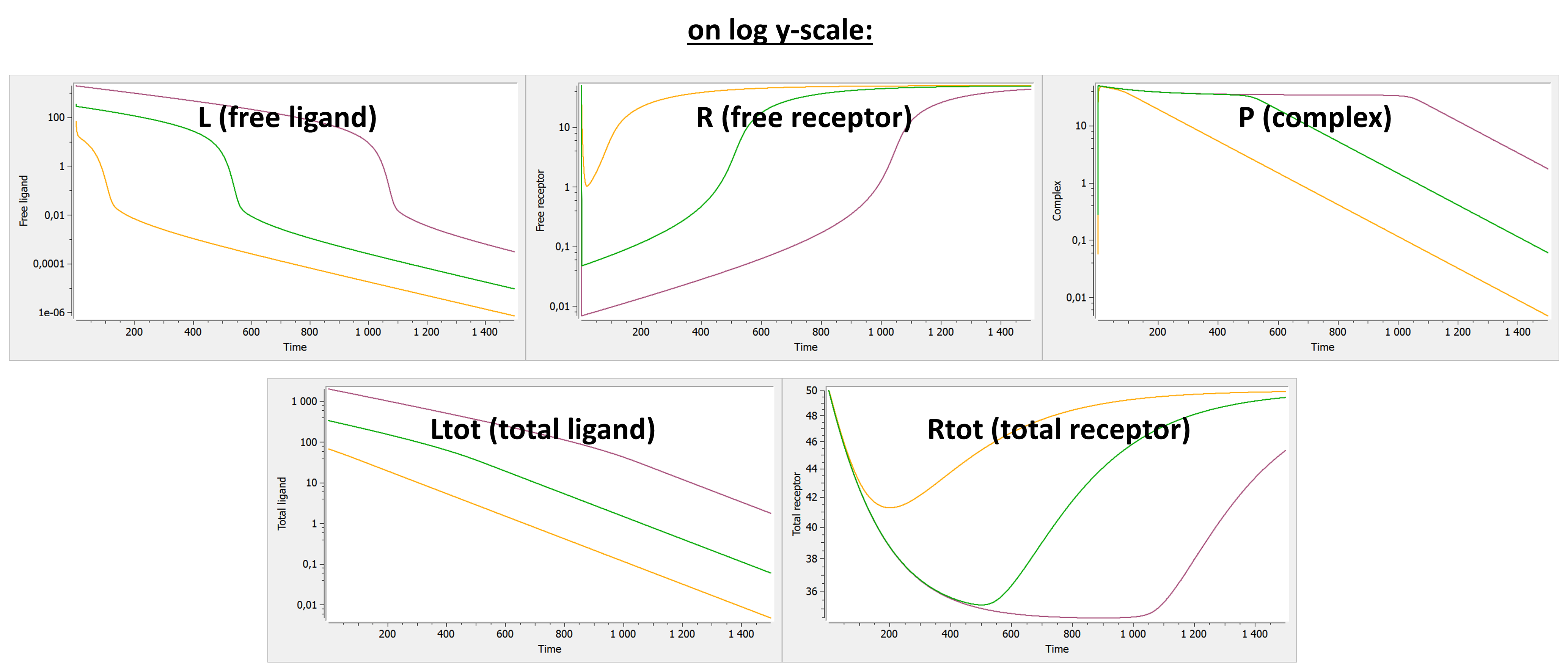
The original TMDD model and its approximations are useful to capture concentration data that display this kind of shapes, or part of them. Below we first describe the content of the library, then we describe the different models and finally give guidelines to choose an appropriate model.
The TMDD library
The library contains a large number of TMDD models corresponding to different approximations, different administration routes, different parameterizations, and different outputs. In total 608 model files are available. The ordering and naming convention permits to easily browse through the list. The file names follow the pattern below:
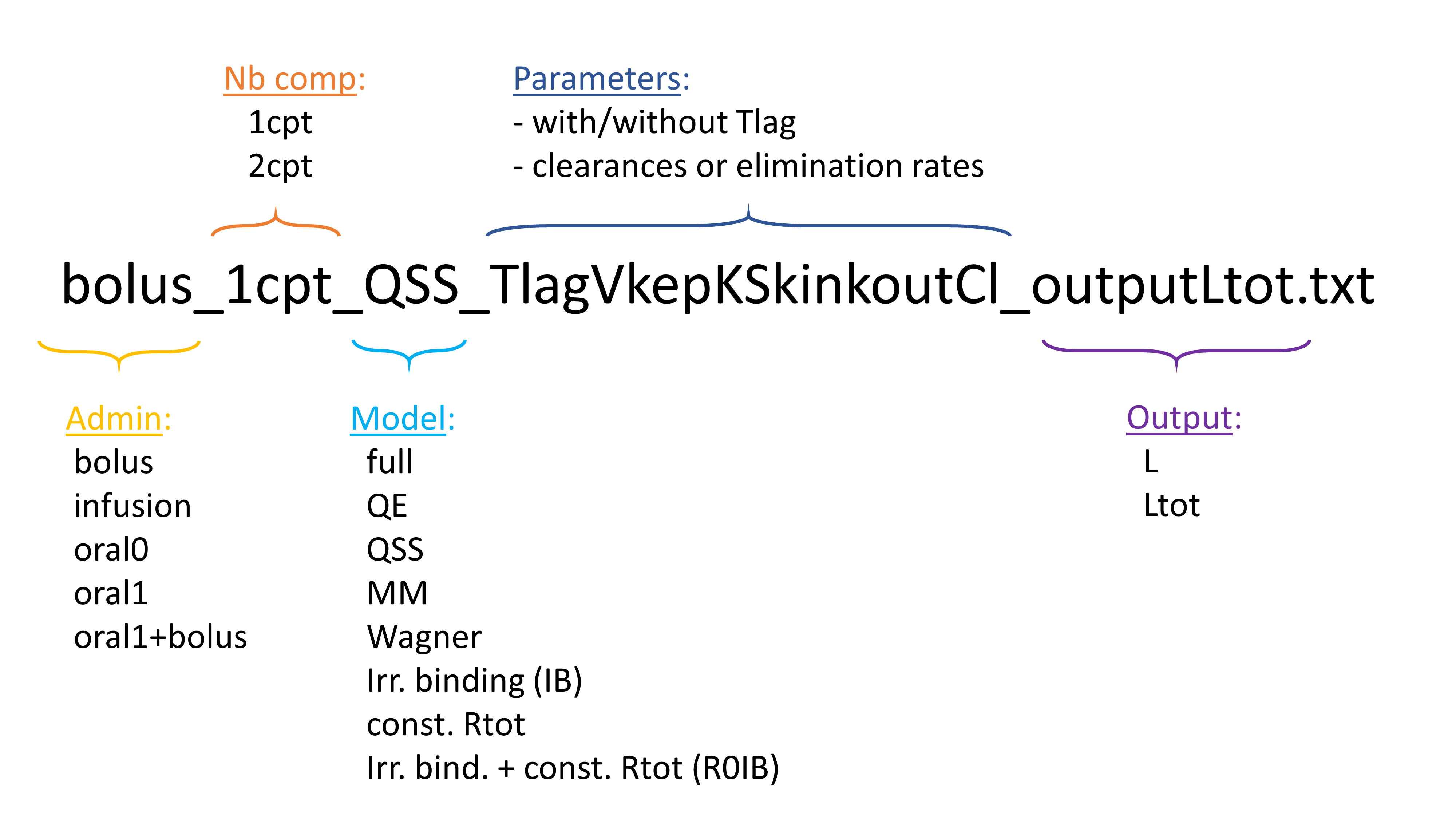
Administration
Five different types of administrations are possible:
- bolus: iv bolus
- infusion: infusion with rate or infusion duration given in the data set (column RATE or TINF)
- oral0: zero-order absorption, with parameter Tk0 for the duration
- oral1: first-order absorption, with parameter ka
- oral1+bolus: first-order absorption or bolus depending on the dose. Bolus doses must be tagged with ADM=1 in the data set and first-order doses (oral or subcutaneous for instance) with ADM=2.
Note that repeated administrations are also allowed. If combinations other than oral1+bolus are necessary, the model file can be duplicated and modified to include a second administration type. In the model, the administration types are distinguished using the type or adm keyword. In the data set, an ADM column must be present.
Number of compartments
All models are available either with 1 compartment or with 2 compartments (central and peripheral). The impact on the model behavior will be detailed in the next section.
Models (approximations)
Beside the original full TMDD system of equations, several approximations have been derived, corresponding to different limit cases. The hierarchy of these approximations and their impact on the model behavior will be detailed in the next section.
Parameters
The list of parameters is mentioned in each file name. The naming convention follows Gibiansky et al. (2008), JPP 35(5). We use the parameters (ksyn, R0) instead of (ksyn, kdeg), and (kon, KD) instead of (kon, koff) because they allow an easier initialization of the parameters. For the elimination and peripheral compartment, two parameterizations are possible, either using clearances or using rates. In addition, a parameter Tlag is available to introduce a time lag for the administration.
Outputs
The model outputs will be matched to the observed data. If only the free ligand L, or the total ligand Ltot have been measured, the files ending with ‘outputL’ and ‘outputLtot’ can be used respectively. If one or several other entities have been measured, the model files must be adapted to output one or several variables in the MARKDOWN_HASHe4fdc9890583978ba7811d0e48b55a31MARKDOWN_HASH section.
If several outputs are present, the outputs will be matched by order with the YTYPEs defined in the data set (first model output matched to observations with YTYPE=1, second model output matched to observations with YTYPE=2, etc). For all models except the Michaelis-Menten TMDD model, the available outputs are the following:
- L: free ligand
- R: free target/receptor
- P: free complex
- Ltot: total (free + bound) ligand
- Rtot: total (free + bound) target/receptor
- TO: receptor occupancy (TO=R/Rtot)
- RR: ratio of free receptor to baseline value (RR=R/R0)
For the Michaelis-Menten TMDD model, only the free ligand L is available as output.
Adapting the models for multiple administration types
Except the oral1+bolus, the models from the library are written for only one administration type per data set. However, they can easily be modified to handle several types of administrations.
In the data set, the doses must be associated to an administration identifier in the ADM column. In the example below, the first dose is assigned to ADM=1 and the second to ADM=2. Often the CMT column of Nonmem data sets can simply be tagged as ADM column in Monolix.
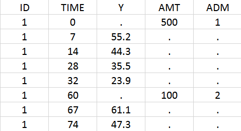
Using the library model files as a template, the user can then create a new model file adapting the depot statements in the PK: block to its need. In the case of iv and sub-cutaneous administrations, one would write:
PK:
depot(adm=1, target=L, p=1/V) ; doses with ADM=1 in the data set, iv bolus
depot(adm=2, target=L, p=1/V, ka) ; doses with ADM=2 in the data set, first-order absorption with rate ka
For each dose, the depot macro will apply a bolus or first-order input rate to the target L, depending on the ADM identifier of the data set.
Do not forget to include the additional parameters into the MARKDOWN_HASH8d060b1490f65f1cab71b12b99c2985eMARKDOWN_HASH statement.
Download
You can download the library here. All the models are text files. To use it, extract all in a TMDD folder for example.
Overview of the model hierarchy
The figure below gives an overview of the different models, their parameter and the resulting typical concentration-time curve for the free ligand. The assumptions leading from one approximation to another one are also depicted.
The plots represent typical concentration-time curves in log-scale for the free ligand L. The graphics comes from a Mlxplore project defined below. The arrows depict the degrees of flexibility: curved arrows denote that the angle can be changed, while straight arrows denote that the curve can be shifted.
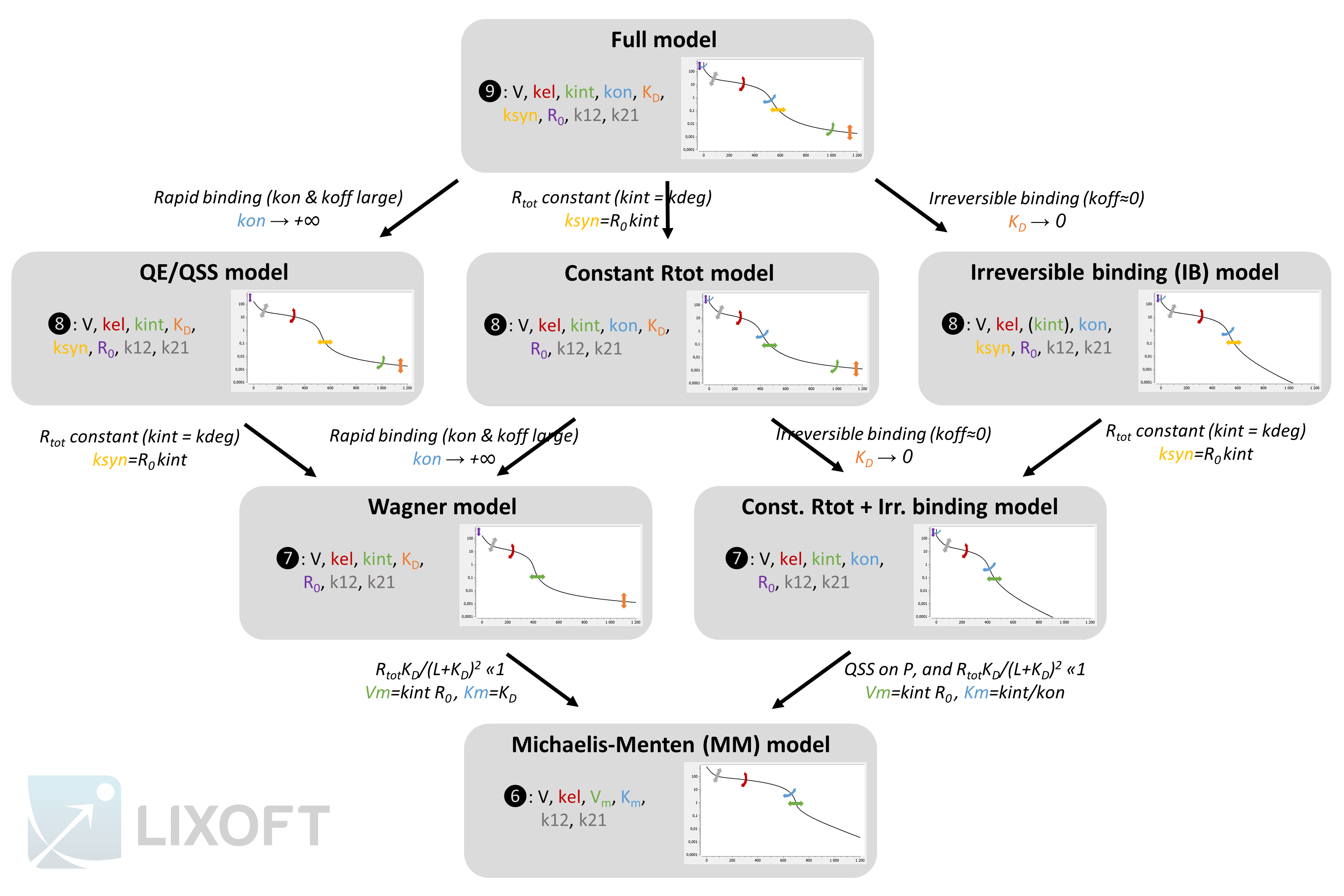
You can use this scheme but you need to cite Lixoft when using it (high quality pdf scheme here). A few comments to better understand the scheme:
- The QE and QSS models are shown together because their system of equations is the same. However the QSS model is derived from the full model using a quasi steady-state assumption. In this case, the name of the new parameter is
.
- The parameters for the second compartment (k12 and k21) influence the non-linear concentration decrease in phase 2, but also the slopes of phase 3 and 4 (which is not depicted for clarity). In the models that lack flexibility in phase 4 (IB, Wagner, MM and const Rtot+IB), some flexibility is present due to k12 and k21 but it is tightly related to the shape of the non-linearity in phase 2.
- In the first and second rows of models, kint influences the slope of phase 4. On the opposite, in the third and fourth rows, kint influences the start time of phase 3, which was previously influenced by ksyn. Note that because
and
, ksyn and kint are related via
.
- The circled numbers represent the number of parameters for a two compartment model. In case of a one compartment model, the number of parameters would be reduced by two. With a single compartment, the phase 2 would be linear. In addition, phase 4 would be completely missing for the IB, MM and const. Rtot+IB models. These curves can be seen in the detailed description section.
- In the IB model, the kint parameter has no influence on the free ligand concentration L, but it has on the total ligand concentration Ltot. If only the free ligand concentration L is measured, the IB and the const. Rtot+IB models are equivalent.
 .
. .
.An Mlxplore project allowing to explore simultaneously the behavior of the seven models, for all entities, is available here. Uncomment the lines in the sections <OUTPUT> and <RESULTS> to switch from L to other entities. Uncomment the lines in section <DESIGN> to compare the impact of several dose amounts. Set k12=0 to explore the behavior of a one compartment model. Note that a saturation at 1e-6 was added for some models to avoid infinitely small values in the one compartment case. In the “graphic” tab, in section “Axes”, you can choose between linear or log scale. To change the type of administration, you can adapt the depot macro, add the additional parameter(s) to the input list and give a reference parameter value in the <PARAMETER> section.
Detailed description of the models
For clarity reasons, each model has its own dedicated page. All the links are below.
- Full model
- Rapid binding (QE) and quasi steady-state (QSS) models
- Constant Rtot model
- Irreversible binding model
- Wagner model
- Constant Rtot + irreversible binding model
- Michaelis-Menten (MM) model
Guidelines to choose an appropriate model
The guidelines are given on a separate webpage.
Typical parameters for TMDD
Following the PAGE talk by Leonid Gibiansky, the table below summarizes the typical TMDD parameters, their distribution, their usual range of values, their units, as well as possible covariates: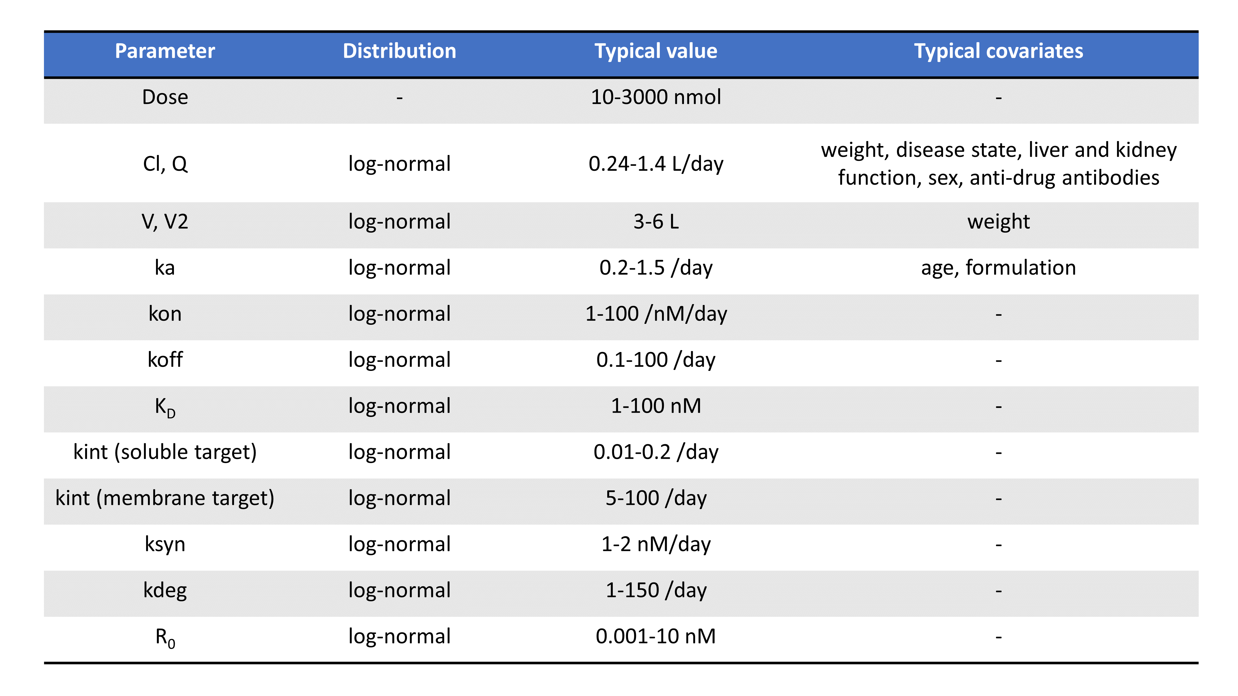
Note that parameters related to the binding (such as Km, KD, kon, koff) depends on the molecule’s chemical properties and are less likely to vary from individual to individual, compared to volumes or parameters that depend on enzyme levels such as kel for instance.
An extensive literature review of parameter values for monoclonal antibodies is also presented in Le Dirks (2010).
Examples of molecules
The table below presents a few examples of molecules displaying TMDD. Biologics are typical candidates for TMDD but small molecules can also display TMDD kinetics. The models used to describe the kinetics of these molecules range from simple MM TMDD models with one compartment to the full TMDD model with 2 compartments.
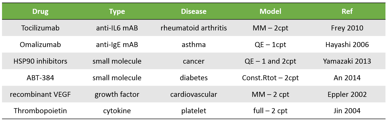
Extensions to more complex TMDD models
In this section, we propose links to resources to extend the proposed library of models to more complex TMDD models. The user who wishes to incorporate these extensions can use the library model files as a starting point.
PK/PD modeling
The mechanistic approach used in TMDD models makes it easy to extend the PK model to a PK/PD model and assume that the pharmacological effect is proportional to the concentration of the drug-receptor complex or to the target occupancy. PK/PD models for molecules displaying TMDD kinetics are for instance presented in Bauer et al. (1999), JPB 27(4), or in Mager et al. (2003), JPET 307(3).
Prediction of human PK from animal data
The prediction of the human PK of drugs is a key step for the accurate estimation of doses for first in human clinical trials. Two approaches are often used: allometric scaling and physiologically-based PK models.
Inter-species allometric scaling
To predict human pharmacokinetic parameters values from animal data, inter-species scaling is often used for small molecules. In the most common approach, the PK parameters are related to the body-weight using a power law. This approach is also often used for biologics, although possible species difference in the target must be kept in mind (Glassmann et al. (2016), JPP 43(4)). Successes and limitations are for instance presented in Kagan et al. (2010, Pharm Res 27), and Dong et al. (2011, Clin Pharm 50(2)).
Physiologically-based TMDD models
Physiologically-based pharmacokinetic (PBPK) models extend typical PK models to more compartments that represent the different organs or tissues of the body, with interconnections corresponding to blood flows. The incorporation of the body’s anatomy and physiology in a more detailed way makes it possible to predict human PK by adapting the volumes and flows of the animal body to those of the human body. A quite generic PBPK model for molecules displaying TMDD kinetics is presented in Glassman et al. (2016), JPP 43(3), and applied to four monoclonal antibodies. For three of them, the model could well predict the human PK.
Ligand facilitated target removal
To use ligand facilitated target removal (LFTR) model, presented in Peletier et al. (2021), a small change needs to be made to the full TMDD model available in the TMDD library. ODE line describing ligand behavior needs to be changed to ddt_L = -kel*L – kon*L*R + (koff+kint)*P.
More complex PK TMDD models
The full TMDD model presented here contains a number of implicit assumptions such as no binding in peripheral tissues, only one target, only one ligand, and no presence of endogenous drug amounts. Models have been proposed that alleviate these hypotheses. They are reviewed in Dua et al. (2015), CPT:PSP 4(6) and we here propose a short list of possible extensions:
- binding in the tissue compartment: Lowe et al. (2010), BCPT 106(3).
- multiple targets: Gibiansky et al. (2010), JPP 37(4).
- receptor recycling: Krippendorff et al. (2009), JPP 36.
- immune response: Perez-Ruixo et al. (2013), AAPS journal 15(1).
- drug-drug interactions: Yan et al. (2012), JPP 39(5), and Koch et al. (2017), JPP 44(1).
- endogenous drug present: Koch et al. (2017), JPP.
8.5.1.Full TMDD model
We here present the system of equation corresponding to the original (full) TMDD model, as well as the model behavior.
Equations
The first TMDD model has been proposed in Mager & Jusko (2001), JPP 28(6). The equations read:
}{V} - k_{\textrm{el}} \: L - k_{\textrm{on}}\:L\:R + k_{\textrm{off}}\:P \\ \dfrac{dR}{dt} &=& k_{\textrm{syn}} - k_{\textrm{deg}}\:R - k_{\textrm{on}}\:L\:R + k_{\textrm{off}}\:P \\ \dfrac{dP}{dt} &=& k_{\textrm{on}}\:L\:R - k_{\textrm{off}}\:P - k_{\textrm{int}}\:P \end{array}")
with L the concentration of the ligand in plasma, R the concentration of the target/receptor, and P the concentration of the complex. V is the volume of the central compartment for the ligand, kel the linear elimination rate for the ligand, kon the binding rate, koff the dissociation rate, ksyn the synthesis rate for the target/receptor, kdeg its degradation rate, and kint the degradation rate of the complex. In(t) represents the input function, corresponding to the input rate (amount per unit time) of the ligand into the central compartment due to the ligand administration.
In the library model file, a slightly different parameterization is used using 

If in addition the ligand can distribute to peripheral tissues, a second compartment can be added, leading to:
}{V} - k_{\textrm{el}} \: L - k_{\textrm{on}}\:L\:R + k_{\textrm{off}}\:P - k_{\textrm{12}}\:L + k_{\textrm{21}}\:A/V \\ \dfrac{dR}{dt} &=& k_{\textrm{syn}} - k_{\textrm{deg}}\:R - k_{\textrm{on}}\:L\:R + k_{\textrm{off}}\:P \\ \dfrac{dP}{dt} &=& k_{\textrm{on}}\:L\:R - k_{\textrm{off}}\:P - k_{\textrm{int}}\:P \\ \dfrac{dA}{dt} &=& k_{\textrm{12}}\:L\:V - k_{\textrm{21}}\:A\end{array}")
with A the amount of ligand in peripheral tissues, k12 the rate of transfert from central to peripheral, and k21 the rate in the opposite direction.
The main assumptions of this model are the following (Gibiansky et al. PAGE 2011 talk):
- the binding of the ligand to the target is simple, not cooperative
- binding occurs only in the central compartment
- target and complex do not diffuse to peripheral compartments
- internalized ligand-receptor complexes are not recycled
Model properties
To better understand the properties of such a model, we propose to explore the typical concentration-time curves of this model and the influence of the parameter values. We will focus on the concentration-time curve of the free ligand after a bolus dose, while the other species can be investigated by the reader using the provided Mlxplore project files. The vignettes below explicit the impact of each parameter on the typical free ligand concentration-time curve:
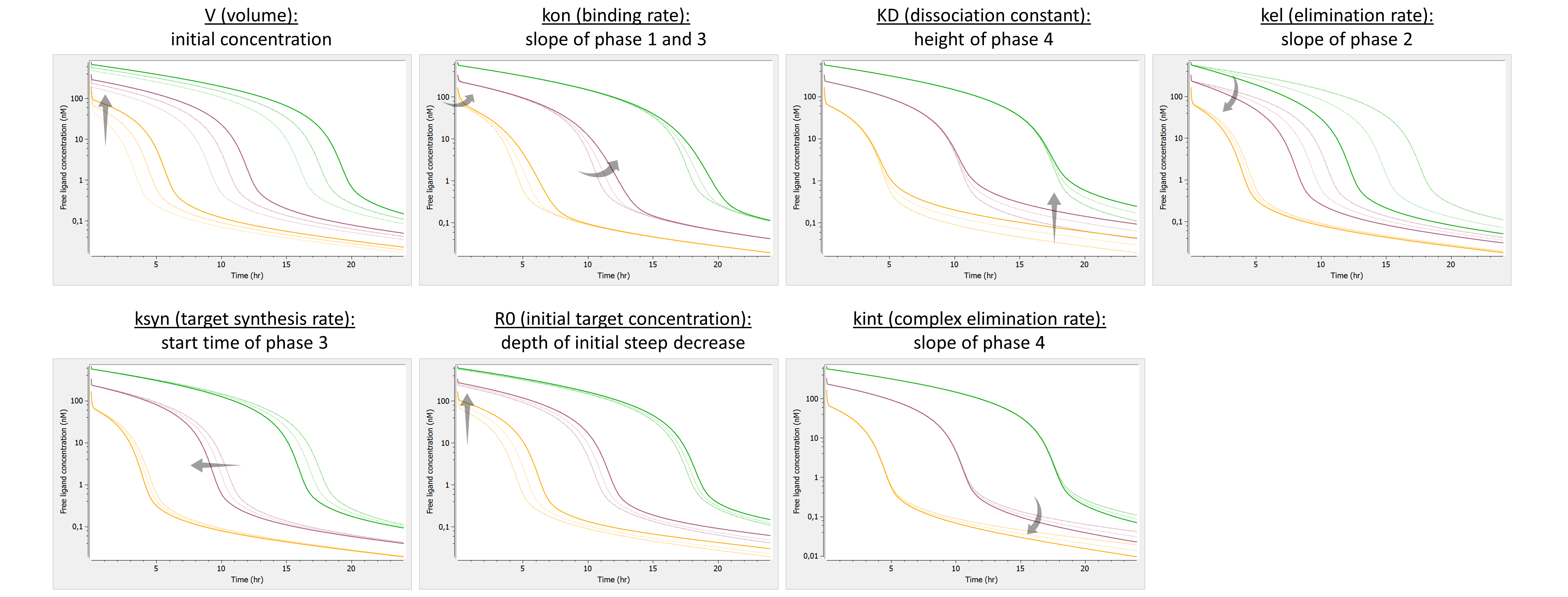
The effects are summarized below:
 For every phase of the concentration-time curve, there exists a parameter to modify it. This is in contrast with the various approximations that lack flexibility for one or several phases of the curve.
Model with 2 compartments
If a second compartment is added, the shape is modified in the following way. Note that kon has been chosen large (very steep phase 1), to better focus on phase 2, where k12 and k21 have their main effect.
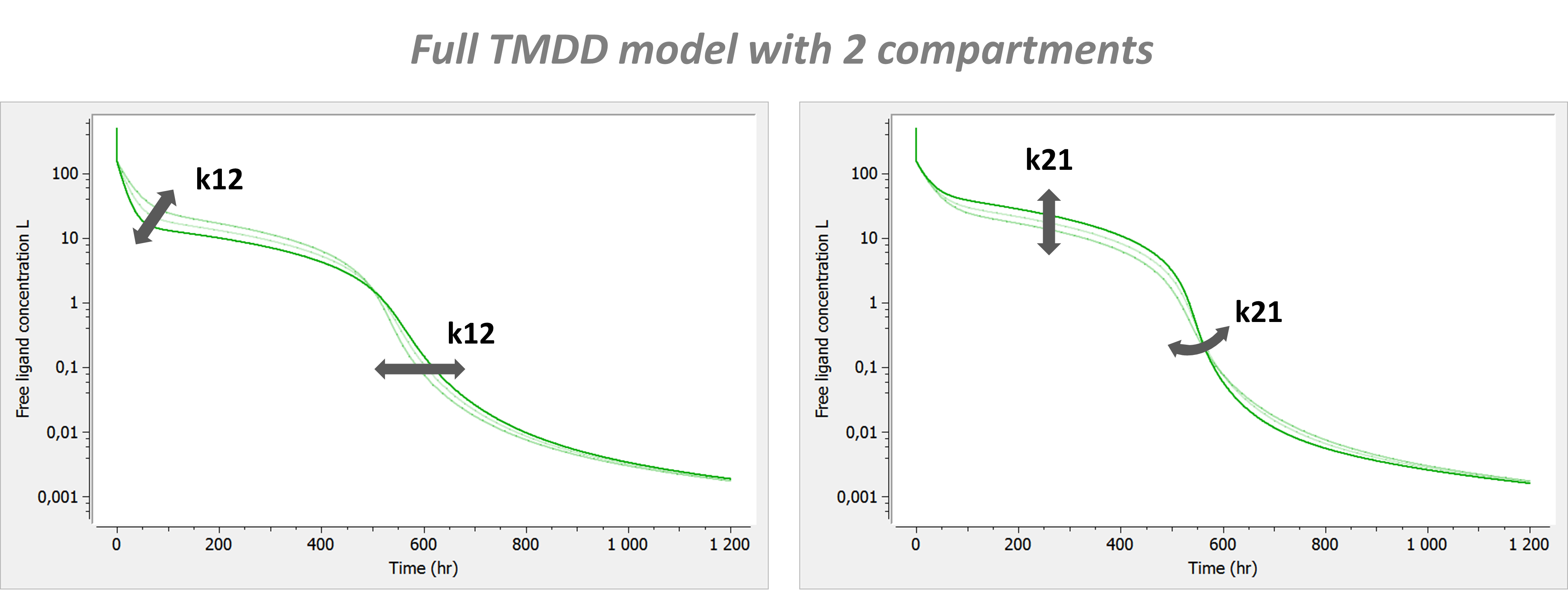
Click here to go back to main TMDD page.
Detailed description of all the models
8.5.2.Rapid binding (QE) and quasi steady-state (QSS) TMDD models
We here present the system of equation corresponding to the QE and QSS TMDD models, as well as the model behavior.
Rapid binding equations
The steep initial decrease (Phase 1) of the free ligand concentration in the full model usually occurs on a very short time-scale (minutes to hours) compared to the other phases (elimination over days or weeks). If the acquired data starts only after this initial phase, the parameters associated with the binding (especially kon) may not be identifiable. This is why the rapid-binding (also called quasi-equilibrium) approximation has been proposed.
The first derivation has been detailed in Mager & Krzyzanski (2005), Pharm Res 22(10), while a more mathematically rigorous derivation can be found in Koch et al. (2016). JPP. In brief, it is assumed that binding and dissociation of the ligand and target is much more rapid than the other processes, such that the free ligand, free receptor and the complex are at quasi-equilibrium: 


![\begin{array}{ccl} \dfrac{dL_{\textrm{tot}}}{dt} &=& \dfrac{\textrm{In}(t)}{V} - k_{\textrm{int}} \: L_{\textrm{tot}} - (k_{\textrm{el}}-k_{\textrm{int}})L \\ \dfrac{dR_{\textrm{tot}}}{dt} &=& k_{\textrm{syn}} - k_{\textrm{deg}}\:R_{\textrm{tot}} - (k_{\textrm{int}}-k_{\textrm{deg}})(L_{\textrm{tot}}-L) \\ L&=&\frac{1}{2}\left[ (L_{\textrm{tot}}-R_{\textrm{tot}}-K_D)+\sqrt{(L_{\textrm{tot}}-R_{\textrm{tot}}-K_D)^2+4K_DL_{\textrm{tot}}}\right] \end{array}](http://s0.wp.com/latex.php?latex=%5Cbegin%7Barray%7D%7Bccl%7D%C2%A0%5Cdfrac%7BdL_%7B%5Ctextrm%7Btot%7D%7D%7D%7Bdt%7D+%26%3D%26+%5Cdfrac%7B%5Ctextrm%7BIn%7D%28t%29%7D%7BV%7D+-+k_%7B%5Ctextrm%7Bint%7D%7D+%5C%3A%C2%A0L_%7B%5Ctextrm%7Btot%7D%7D+-+%28k_%7B%5Ctextrm%7Bel%7D%7D-k_%7B%5Ctextrm%7Bint%7D%7D%29L+%5C%5C+%C2%A0%5Cdfrac%7BdR_%7B%5Ctextrm%7Btot%7D%7D%7D%7Bdt%7D+%26%3D%26+k_%7B%5Ctextrm%7Bsyn%7D%7D+-+k_%7B%5Ctextrm%7Bdeg%7D%7D%5C%3AR_%7B%5Ctextrm%7Btot%7D%7D+-+%C2%A0%28k_%7B%5Ctextrm%7Bint%7D%7D-k_%7B%5Ctextrm%7Bdeg%7D%7D%29%28L_%7B%5Ctextrm%7Btot%7D%7D-L%29+%C2%A0%5C%5C+L%26%3D%26%5Cfrac%7B1%7D%7B2%7D%5Cleft%5B+%28L_%7B%5Ctextrm%7Btot%7D%7D-R_%7B%5Ctextrm%7Btot%7D%7D-K_D%29%2B%5Csqrt%7B%28L_%7B%5Ctextrm%7Btot%7D%7D-R_%7B%5Ctextrm%7Btot%7D%7D-K_D%29%5E2%2B4K_DL_%7B%5Ctextrm%7Btot%7D%7D%7D%5Cright%5D+%5Cend%7Barray%7D&bg=ffffff&fg=000&s=0.5 "\begin{array}{ccl} \dfrac{dL_{\textrm{tot}}}{dt} &=& \dfrac{\textrm{In}(t)}{V} - k_{\textrm{int}} \: L_{\textrm{tot}} - (k_{\textrm{el}}-k_{\textrm{int}})L \\ \dfrac{dR_{\textrm{tot}}}{dt} &=& k_{\textrm{syn}} - k_{\textrm{deg}}\:R_{\textrm{tot}} - (k_{\textrm{int}}-k_{\textrm{deg}})(L_{\textrm{tot}}-L) \\ L&=&\frac{1}{2}\left[ (L_{\textrm{tot}}-R_{\textrm{tot}}-K_D)+\sqrt{(L_{\textrm{tot}}-R_{\textrm{tot}}-K_D)^2+4K_DL_{\textrm{tot}}}\right] \end{array}")
As before, V is the volume of the central compartment for the ligand, kel the linear elimination rate for the ligand, KD the dissociation rate, ksyn the synthesis rate for the target/receptor, kdeg its degradation rate, and kint the degradation rate of the complex. In(t) represents the input function, corresponding to the input rate (amount per unit time) of the ligand into the central compartment due to the ligand administration.
In the library model file, a slightly different parameterization is used using
The complex concentration can be calculated via 
")
As for the full model, the system can be extended with a peripheral compartment, leading to:
![\begin{array}{ccl} \dfrac{dL_{\textrm{tot}}}{dt} &=& \dfrac{\textrm{In}(t)}{V} - k_{\textrm{int}} \: L_{\textrm{tot}} - (k_{\textrm{el}}-k_{\textrm{int}})L - k_{\textrm{12}}\:L + k_{\textrm{21}}\:A/V \\ \dfrac{dR_{\textrm{tot}}}{dt} &=& k_{\textrm{syn}} - k_{\textrm{deg}}\:R_{\textrm{tot}} - (k_{\textrm{int}}-k_{\textrm{deg}})(L_{\textrm{tot}}-L) \\ \dfrac{dA}{dt} &=& k_{\textrm{12}}\:L\:V - k_{\textrm{21}}\:A \\ L&=&\frac{1}{2}\left[ (L_{\textrm{tot}}-R_{\textrm{tot}}-K_D)+\sqrt{(L_{\textrm{tot}}-R_{\textrm{tot}}-K_D)^2+4K_DL_{\textrm{tot}}}\right] \end{array}](http://s0.wp.com/latex.php?latex=%5Cbegin%7Barray%7D%7Bccl%7D%C2%A0%5Cdfrac%7BdL_%7B%5Ctextrm%7Btot%7D%7D%7D%7Bdt%7D+%26%3D%26+%5Cdfrac%7B%5Ctextrm%7BIn%7D%28t%29%7D%7BV%7D+-+k_%7B%5Ctextrm%7Bint%7D%7D+%5C%3A%C2%A0L_%7B%5Ctextrm%7Btot%7D%7D+-+%28k_%7B%5Ctextrm%7Bel%7D%7D-k_%7B%5Ctextrm%7Bint%7D%7D%29L+-+k_%7B%5Ctextrm%7B12%7D%7D%5C%3AL+%2B+k_%7B%5Ctextrm%7B21%7D%7D%5C%3AA%2FV+%5C%5C+%C2%A0%5Cdfrac%7BdR_%7B%5Ctextrm%7Btot%7D%7D%7D%7Bdt%7D+%26%3D%26+k_%7B%5Ctextrm%7Bsyn%7D%7D+-+k_%7B%5Ctextrm%7Bdeg%7D%7D%5C%3AR_%7B%5Ctextrm%7Btot%7D%7D+-+%C2%A0%28k_%7B%5Ctextrm%7Bint%7D%7D-k_%7B%5Ctextrm%7Bdeg%7D%7D%29%28L_%7B%5Ctextrm%7Btot%7D%7D-L%29+%5C%5C+%5Cdfrac%7BdA%7D%7Bdt%7D+%26%3D%26%C2%A0k_%7B%5Ctextrm%7B12%7D%7D%5C%3AL%5C%3AV+-+k_%7B%5Ctextrm%7B21%7D%7D%5C%3AA+%C2%A0%5C%5C+L%26%3D%26%5Cfrac%7B1%7D%7B2%7D%5Cleft%5B+%28L_%7B%5Ctextrm%7Btot%7D%7D-R_%7B%5Ctextrm%7Btot%7D%7D-K_D%29%2B%5Csqrt%7B%28L_%7B%5Ctextrm%7Btot%7D%7D-R_%7B%5Ctextrm%7Btot%7D%7D-K_D%29%5E2%2B4K_DL_%7B%5Ctextrm%7Btot%7D%7D%7D%5Cright%5D+%5Cend%7Barray%7D&bg=ffffff&fg=000&s=0.5 "\begin{array}{ccl} \dfrac{dL_{\textrm{tot}}}{dt} &=& \dfrac{\textrm{In}(t)}{V} - k_{\textrm{int}} \: L_{\textrm{tot}} - (k_{\textrm{el}}-k_{\textrm{int}})L - k_{\textrm{12}}\:L + k_{\textrm{21}}\:A/V \\ \dfrac{dR_{\textrm{tot}}}{dt} &=& k_{\textrm{syn}} - k_{\textrm{deg}}\:R_{\textrm{tot}} - (k_{\textrm{int}}-k_{\textrm{deg}})(L_{\textrm{tot}}-L) \\ \dfrac{dA}{dt} &=& k_{\textrm{12}}\:L\:V - k_{\textrm{21}}\:A \\ L&=&\frac{1}{2}\left[ (L_{\textrm{tot}}-R_{\textrm{tot}}-K_D)+\sqrt{(L_{\textrm{tot}}-R_{\textrm{tot}}-K_D)^2+4K_DL_{\textrm{tot}}}\right] \end{array}")
with A the amount of ligand in peripheral tissues, k12 the rate of transfert from central to peripheral, and k21 the rate in the opposite direction.
Note that the number of parameters has been reduced by one, as kon and koff have been replaced by KD. The behavior of the rapid-binding approximation will be close to the full model behavior if indeed the binding and dissociation reactions are fast compared to the other reactions.
Quasi steady-state equations
The quasi steady-state approximation has been proposed by Gibiansky et al. (2008, JPP 35(5)) for the same reasons as the rapid-binding approximation: lack of identifiability of the full model for typical data sets.
In the QSS approximation, one assumes that the binding rate is balanced by the sum of the dissociation and internalization rates leading to P=0")

Again, it is more convenient to work with the total ligand concentration and the total receptor concentration, and the equations read:
![\begin{array}{ccl} \dfrac{dL_{\textrm{tot}}}{dt} &=& \dfrac{\textrm{In}(t)}{V} - k_{\textrm{int}} \: L_{\textrm{tot}} - (k_{\textrm{el}}-k_{\textrm{int}})L \\ \dfrac{dR_{\textrm{tot}}}{dt} &=& k_{\textrm{syn}} - k_{\textrm{deg}}\:R_{\textrm{tot}} - (k_{\textrm{int}}-k_{\textrm{deg}})(L_{\textrm{tot}}-L) \\ L&=&\frac{1}{2}\left[ (L_{\textrm{tot}}-R_{\textrm{tot}}-K_{SS})+\sqrt{(L_{\textrm{tot}}-R_{\textrm{tot}}-K_{SS})^2+4K_{SS}L_{\textrm{tot}}}\right] \end{array}](http://s0.wp.com/latex.php?latex=%5Cbegin%7Barray%7D%7Bccl%7D%C2%A0%5Cdfrac%7BdL_%7B%5Ctextrm%7Btot%7D%7D%7D%7Bdt%7D+%26%3D%26+%5Cdfrac%7B%5Ctextrm%7BIn%7D%28t%29%7D%7BV%7D+-+k_%7B%5Ctextrm%7Bint%7D%7D+%5C%3A%C2%A0L_%7B%5Ctextrm%7Btot%7D%7D+-+%28k_%7B%5Ctextrm%7Bel%7D%7D-k_%7B%5Ctextrm%7Bint%7D%7D%29L+%5C%5C+%C2%A0%5Cdfrac%7BdR_%7B%5Ctextrm%7Btot%7D%7D%7D%7Bdt%7D+%26%3D%26+k_%7B%5Ctextrm%7Bsyn%7D%7D+-+k_%7B%5Ctextrm%7Bdeg%7D%7D%5C%3AR_%7B%5Ctextrm%7Btot%7D%7D+-+%C2%A0%28k_%7B%5Ctextrm%7Bint%7D%7D-k_%7B%5Ctextrm%7Bdeg%7D%7D%29%28L_%7B%5Ctextrm%7Btot%7D%7D-L%29+%C2%A0%5C%5C+L%26%3D%26%5Cfrac%7B1%7D%7B2%7D%5Cleft%5B+%28L_%7B%5Ctextrm%7Btot%7D%7D-R_%7B%5Ctextrm%7Btot%7D%7D-K_%7BSS%7D%29%2B%5Csqrt%7B%28L_%7B%5Ctextrm%7Btot%7D%7D-R_%7B%5Ctextrm%7Btot%7D%7D-K_%7BSS%7D%29%5E2%2B4K_%7BSS%7DL_%7B%5Ctextrm%7Btot%7D%7D%7D%5Cright%5D+%5Cend%7Barray%7D&bg=ffffff&fg=000&s=0.5 "\begin{array}{ccl} \dfrac{dL_{\textrm{tot}}}{dt} &=& \dfrac{\textrm{In}(t)}{V} - k_{\textrm{int}} \: L_{\textrm{tot}} - (k_{\textrm{el}}-k_{\textrm{int}})L \\ \dfrac{dR_{\textrm{tot}}}{dt} &=& k_{\textrm{syn}} - k_{\textrm{deg}}\:R_{\textrm{tot}} - (k_{\textrm{int}}-k_{\textrm{deg}})(L_{\textrm{tot}}-L) \\ L&=&\frac{1}{2}\left[ (L_{\textrm{tot}}-R_{\textrm{tot}}-K_{SS})+\sqrt{(L_{\textrm{tot}}-R_{\textrm{tot}}-K_{SS})^2+4K_{SS}L_{\textrm{tot}}}\right] \end{array}")
The complex concentration can be calculated via
And with a peripheral compartment, they read:
![\begin{array}{ccl} \dfrac{dL_{\textrm{tot}}}{dt} &=& \dfrac{\textrm{In}(t)}{V} - k_{\textrm{int}} \: L_{\textrm{tot}} - (k_{\textrm{el}}-k_{\textrm{int}})L - k_{\textrm{12}}\:L + k_{\textrm{21}}\:A/V \\ \dfrac{dR_{\textrm{tot}}}{dt} &=& k_{\textrm{syn}} - k_{\textrm{deg}}\:R_{\textrm{tot}} - (k_{\textrm{int}}-k_{\textrm{deg}})(L_{\textrm{tot}}-L) \\ \dfrac{dA}{dt} &=& k_{\textrm{12}}\:L\:V - k_{\textrm{21}}\:A \\ L&=&\frac{1}{2}\left[ (L_{\textrm{tot}}-R_{\textrm{tot}}-K_{SS})+\sqrt{(L_{\textrm{tot}}-R_{\textrm{tot}}-K_{SS})^2+4K_{SS}L_{\textrm{tot}}}\right] \end{array}](http://s0.wp.com/latex.php?latex=%5Cbegin%7Barray%7D%7Bccl%7D%C2%A0%5Cdfrac%7BdL_%7B%5Ctextrm%7Btot%7D%7D%7D%7Bdt%7D+%26%3D%26+%5Cdfrac%7B%5Ctextrm%7BIn%7D%28t%29%7D%7BV%7D+-+k_%7B%5Ctextrm%7Bint%7D%7D+%5C%3A%C2%A0L_%7B%5Ctextrm%7Btot%7D%7D+-+%28k_%7B%5Ctextrm%7Bel%7D%7D-k_%7B%5Ctextrm%7Bint%7D%7D%29L+-+k_%7B%5Ctextrm%7B12%7D%7D%5C%3AL+%2B+k_%7B%5Ctextrm%7B21%7D%7D%5C%3AA%2FV+%5C%5C+%C2%A0%5Cdfrac%7BdR_%7B%5Ctextrm%7Btot%7D%7D%7D%7Bdt%7D+%26%3D%26+k_%7B%5Ctextrm%7Bsyn%7D%7D+-+k_%7B%5Ctextrm%7Bdeg%7D%7D%5C%3AR_%7B%5Ctextrm%7Btot%7D%7D+-+%C2%A0%28k_%7B%5Ctextrm%7Bint%7D%7D-k_%7B%5Ctextrm%7Bdeg%7D%7D%29%28L_%7B%5Ctextrm%7Btot%7D%7D-L%29+%5C%5C+%5Cdfrac%7BdA%7D%7Bdt%7D+%26%3D%26%C2%A0k_%7B%5Ctextrm%7B12%7D%7D%5C%3AL%5C%3AV+-+k_%7B%5Ctextrm%7B21%7D%7D%5C%3AA+%C2%A0%5C%5C+L%26%3D%26%5Cfrac%7B1%7D%7B2%7D%5Cleft%5B+%28L_%7B%5Ctextrm%7Btot%7D%7D-R_%7B%5Ctextrm%7Btot%7D%7D-K_%7BSS%7D%29%2B%5Csqrt%7B%28L_%7B%5Ctextrm%7Btot%7D%7D-R_%7B%5Ctextrm%7Btot%7D%7D-K_%7BSS%7D%29%5E2%2B4K_%7BSS%7DL_%7B%5Ctextrm%7Btot%7D%7D%7D%5Cright%5D+%5Cend%7Barray%7D&bg=ffffff&fg=000&s=0.5 "\begin{array}{ccl} \dfrac{dL_{\textrm{tot}}}{dt} &=& \dfrac{\textrm{In}(t)}{V} - k_{\textrm{int}} \: L_{\textrm{tot}} - (k_{\textrm{el}}-k_{\textrm{int}})L - k_{\textrm{12}}\:L + k_{\textrm{21}}\:A/V \\ \dfrac{dR_{\textrm{tot}}}{dt} &=& k_{\textrm{syn}} - k_{\textrm{deg}}\:R_{\textrm{tot}} - (k_{\textrm{int}}-k_{\textrm{deg}})(L_{\textrm{tot}}-L) \\ \dfrac{dA}{dt} &=& k_{\textrm{12}}\:L\:V - k_{\textrm{21}}\:A \\ L&=&\frac{1}{2}\left[ (L_{\textrm{tot}}-R_{\textrm{tot}}-K_{SS})+\sqrt{(L_{\textrm{tot}}-R_{\textrm{tot}}-K_{SS})^2+4K_{SS}L_{\textrm{tot}}}\right] \end{array}")
Notice that this system of equation is exactly the same as for the rapid binding approximation. The only difference is that the QSS approximation uses 

Model properties
We investigate the influence of each parameter on the typical free ligand concentration-time shape for several dose amounts (bolus administration).
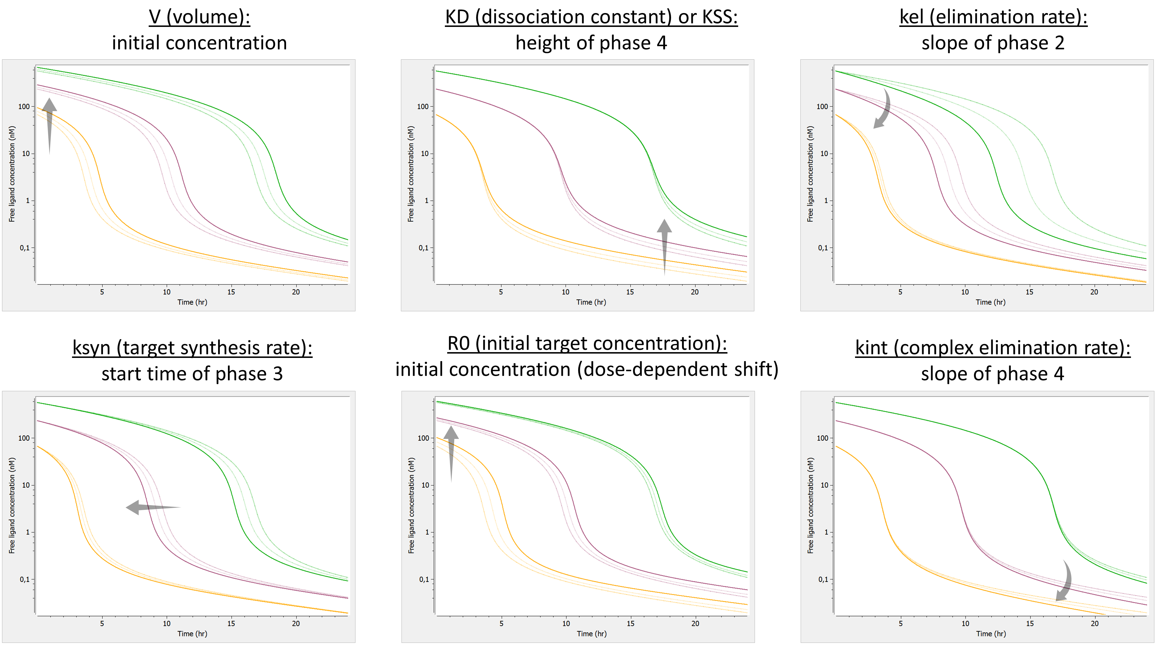
Here is the summary figure:
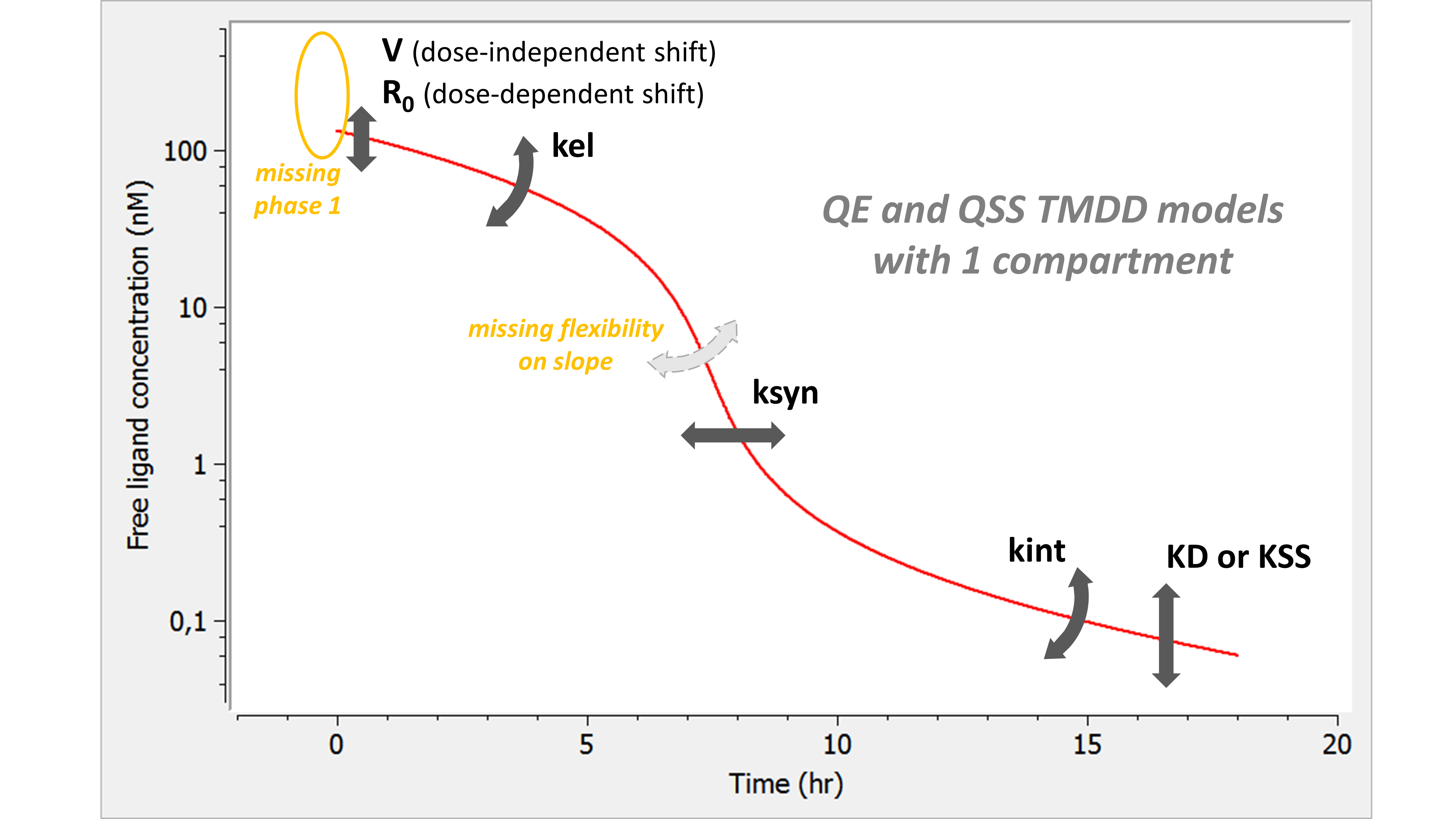
The phase 1 is completely missing. Indeed, as the binding is assumed infinitely fast, part of the ligand binds immediately to the receptor. In addition, the slope of phase 3 is now fixed with none of the parameters having an influence on it.
Note also that both V and R0 impact the initial concentration. However, whereas a change in V leads to the same shift of the initial concentration for all doses (on a linear scale), a change in R0 shifts the initial concentration of low doses more. If the tested doses do not range over enough orders of magnitude, R0 may be unidentifiable.
Model with 2 compartments
If a second compartment is added, the shape is modified in the following way.
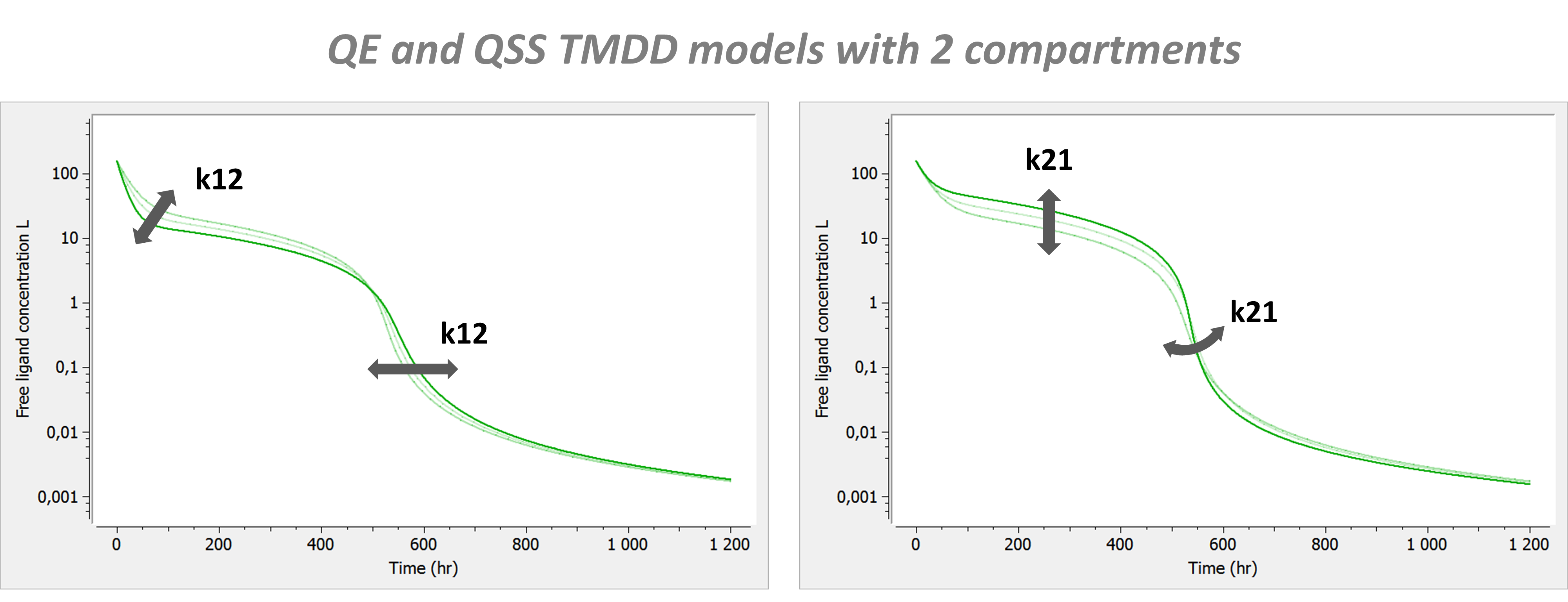
Click here to go back to main TMDD page.
Detailed description of all the models
8.5.3.Constant Rtot TMDD model
We here present the system of equation corresponding to the constant Rtot TMDD model, as well as the model behavior.
Equations
If the degradation rates of the free receptor and the complex are similar (i.e the binding of the ligand to the receptor does not modify the receptor internalization rate), it may not be possible to identify both of them. If both rates are equal (
=R_0=\frac{k_{\textrm{syn}}}{k_{\textrm{deg}}}")
}{V} - (k_{\textrm{el}}+k_{\textrm{on}}R_0) \: L + (k_{\textrm{off}}+k_{\textrm{on}}L)\:P \\ \dfrac{dP}{dt} &=& k_{\textrm{on}}\:R_0\:L - (k_{\textrm{off}} + k_{\textrm{int}} + k_{\textrm{on}}L)\:P \end{array}")
with L the concentration of the ligand in plasma and P the concentration of the complex. V is the volume of the central compartment for the ligand, kel the linear elimination rate for the ligand, kon the binding rate, koff the dissociation rate, R0 the initial receptor concentration, and kint the degradation rate of the complex. In(t) represents the input function, corresponding to the input rate (amount per unit time) of the ligand into the central compartment due to the ligand administration.
In the library model file, a slightly different parameterization is used using
The free receptor concentration can be calculated via 
With 2 compartments for the free ligand, one obtains:
}{V} - (k_{\textrm{el}}+k_{\textrm{on}}R_0) \: L + (k_{\textrm{off}}+k_{\textrm{on}}L)\:P - k_{\textrm{12}}\:L + k_{\textrm{21}}\:A/V \\ \dfrac{dP}{dt} &=& k_{\textrm{on}}\:R_0\:L - (k_{\textrm{off}} + k_{\textrm{int}} + k_{\textrm{on}}L)\:P \\ \dfrac{dA}{dt} &=& k_{\textrm{12}}\:L\:V - k_{\textrm{21}}\:A \end{array}")
with A the amount of ligand in peripheral tissues, k12 the rate of transfert from central to peripheral, and k21 the rate in the opposite direction.
Model properties
We investigate the influence of each parameter on the typical free ligand concentration-time shape for several dose amounts (bolus administration).
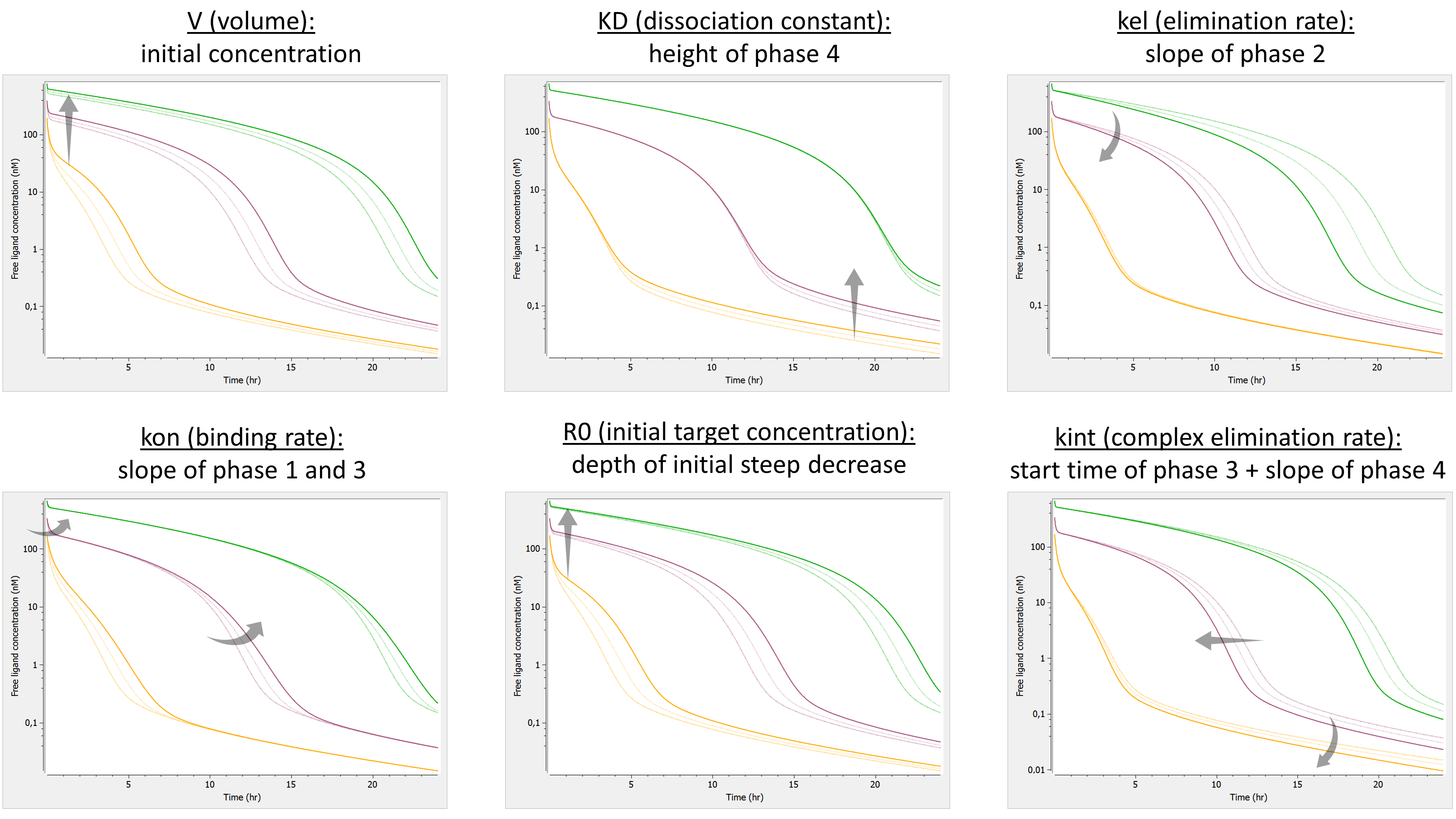
The summary figure is the following:
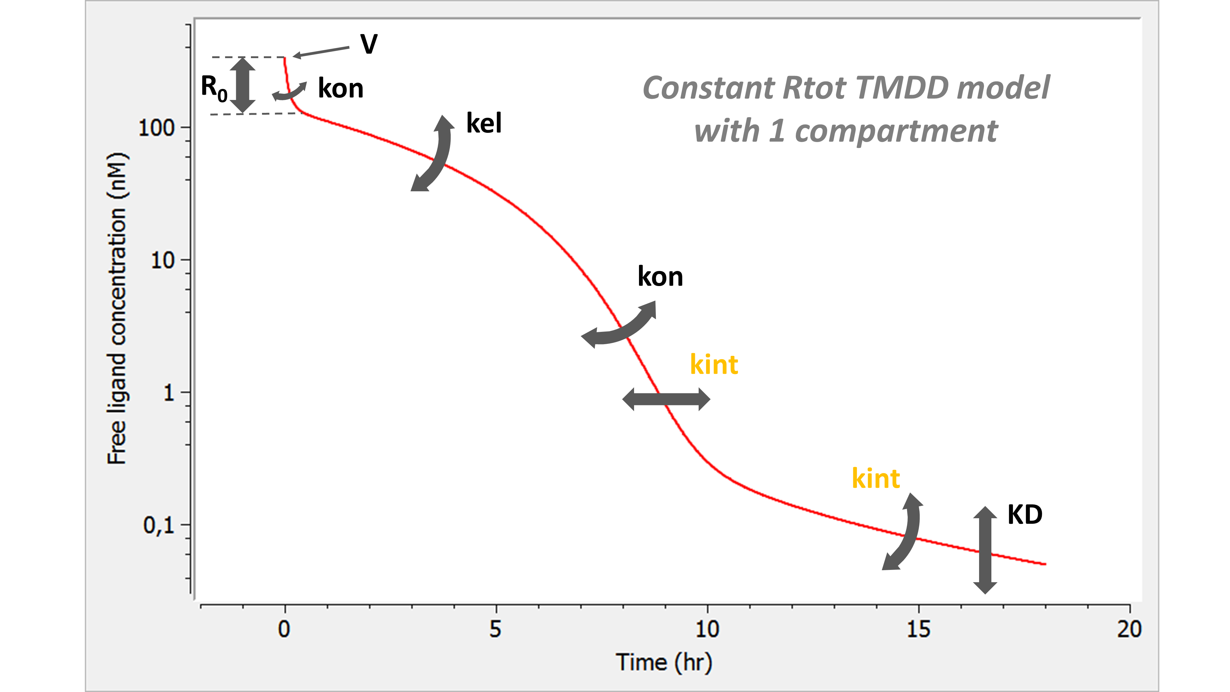
On opposite to the QE/QSS models, the constant Rtot model still captures all four phases of the free ligand concentration-time curve. However, note that because 
Model with 2 compartments
If a second compartment is added, the shape is modified in the following way. Note that kon has been chosen large (very steep phase 1), to better focus on phase 2, where k12 and k21 have their main effect.
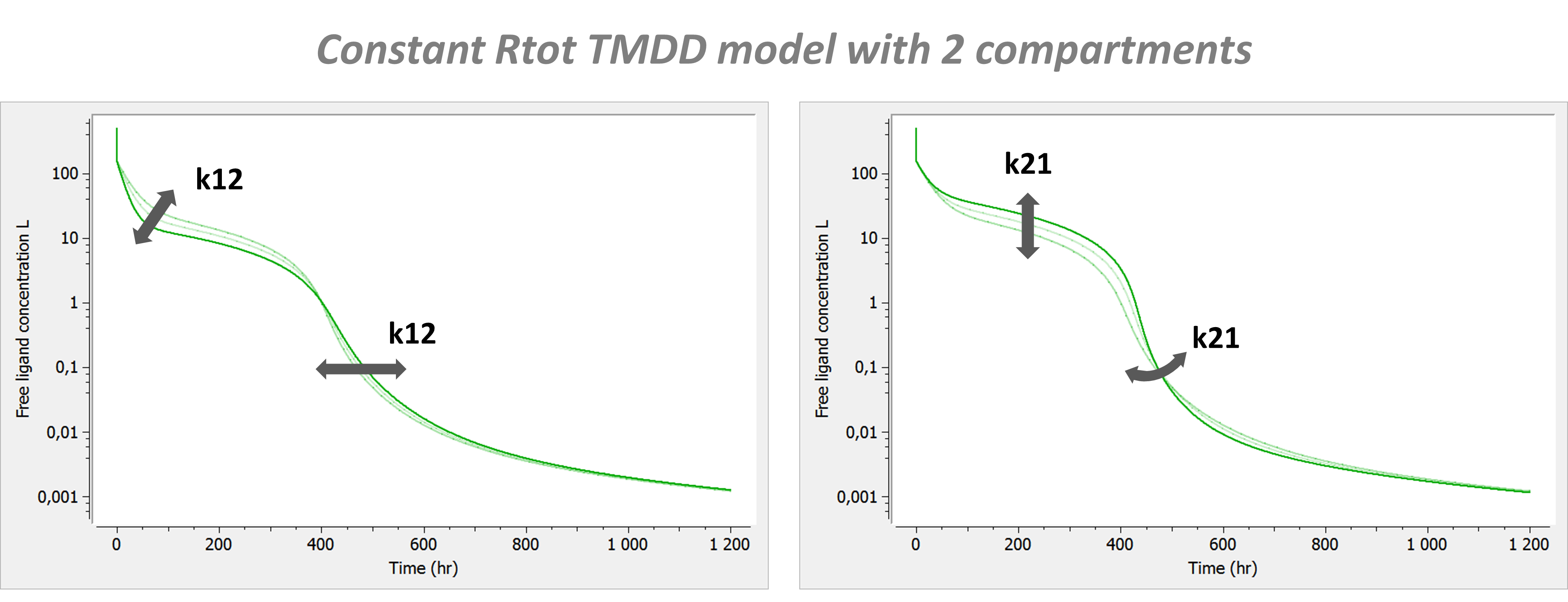
Click here to go back to main TMDD page.
Detailed description of all the models
8.5.4.Irreversible binding TMDD model
We here present the system of equation corresponding to the irreversible binding TMDD model, as well as the model behavior.
Equations
If the binding of the ligand to the receptor is so strong that the dissociation of the ligand from the receptor is negligible, one can consider the binding reaction as irreversible, i.e 
}{V} - k_{\textrm{el}} \: L - k_{\textrm{on}}\:L\:R \\ \dfrac{dR}{dt} &=& k_{\textrm{syn}} - k_{\textrm{deg}}\:R - k_{\textrm{on}}\:L\:R \\ \dfrac{dP}{dt} &=& k_{\textrm{on}}\:L\:R - k_{\textrm{int}}\:P \end{array}")
with L the concentration of the ligand in plasma, R the concentration of the target/receptor, and P the concentration of the complex. V is the volume of the central compartment for the ligand, kel the linear elimination rate for the ligand, kon the binding rate, ksyn the synthesis rate for the target/receptor, kdeg its degradation rate, and kint the degradation rate of the complex. In(t) represents the input function, corresponding to the input rate (amount per unit time) of the ligand into the central compartment due to the ligand administration.
In the library model file, a slightly different parameterization is used using
With a second compartment, one obtains:
}{V} - k_{\textrm{el}} \: L - k_{\textrm{on}}\:L\:R - k_{\textrm{12}}\:L + k_{\textrm{21}}\:A/V \\ \dfrac{dR}{dt} &=& k_{\textrm{syn}} - k_{\textrm{deg}}\:R - k_{\textrm{on}}\:L\:R \\ \dfrac{dP}{dt} &=& k_{\textrm{on}}\:L\:R - k_{\textrm{int}}\:P \\ \dfrac{dA}{dt} &=& k_{\textrm{12}}\:L\:V - k_{\textrm{21}}\:A \end{array}")
with A the amount of ligand in peripheral tissues, k12 the rate of transfert from central to peripheral, and k21 the rate in the opposite direction.
This approximation has one parameter less compared to the full model (koff is fixed to zero). In addition, if only the free ligand L and/or the free receptor R are observed, the equation for P can be removed, leading to:
}{V} - k_{\textrm{el}} \: L - k_{\textrm{on}}\:L\:R \\ \dfrac{dR}{dt} &=& k_{\textrm{syn}} - k_{\textrm{deg}}\:R - k_{\textrm{on}}\:L\:R \end{array}")
In this case, the system has two parameters less then the full system: koff is fixed to zero and kint doesn’t influence the observed species L and R.
Model properties
We investigate the influence of each parameter on the typical free ligand concentration-time shape for several dose amounts.
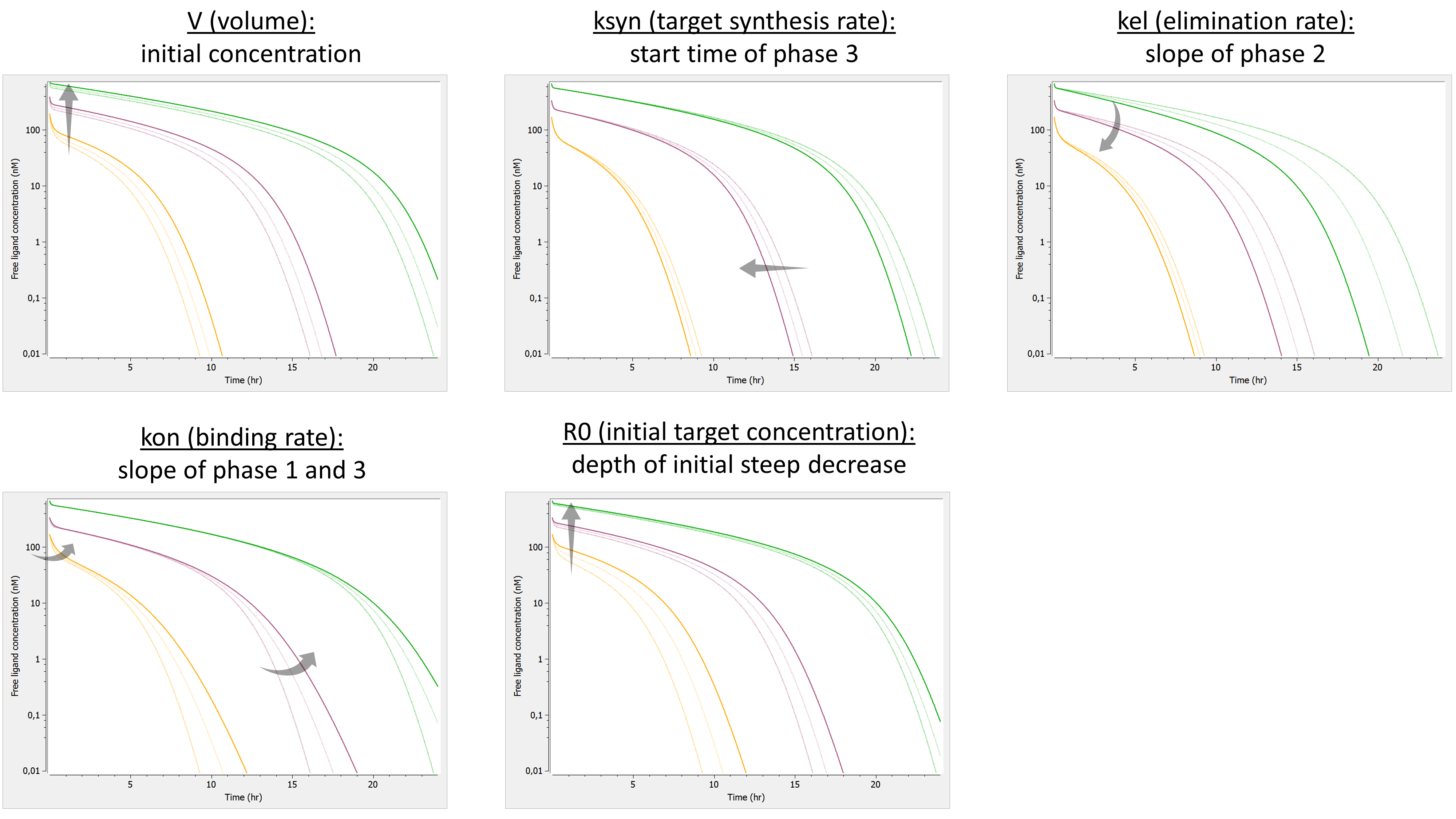
The summary picture is:
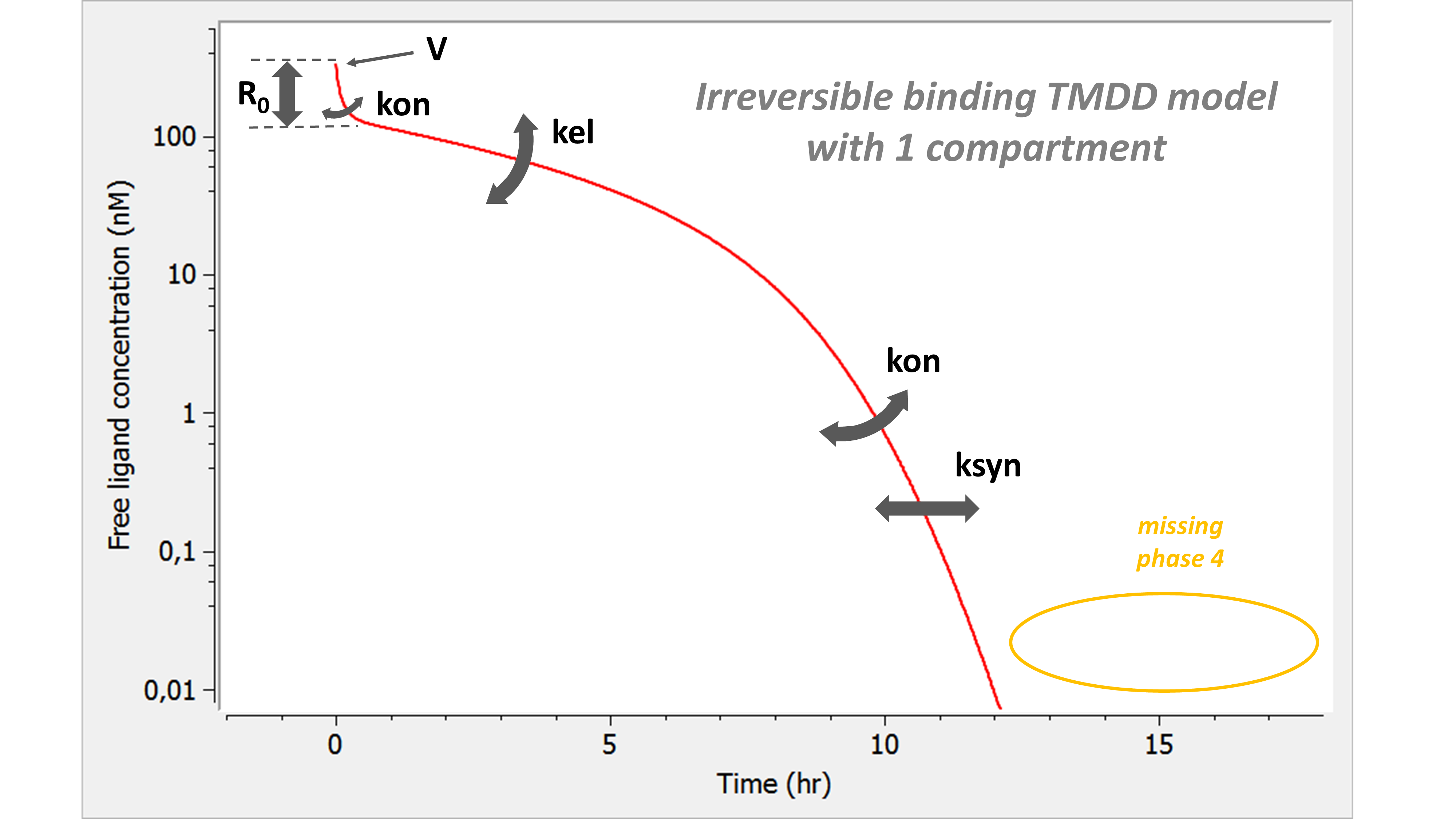
We observe that the phase 4 is completely missing. This approximation can make sense when the phase 4 is below the lower limit of quantification and no data point can be recorded in this zone. If this is the case, KD (or koff) and kint cannot be estimated. Note that if measurements about Ltot, Rtot or P would be available, then the kint parameter might be identifiable.
Model with 2 compartments
If a second compartment is added, the shape is modified in the following way. Note that kon has been chosen large (very steep phase 1), to better focus on phase 2, where k12 and k21 have their main effect.

The introduction of a second compartment permits to recover a phase 4. Its flexibility is limited and linked to the effect of parameters k12 and k21 on phase 2.
Click here to go back to main TMDD page.
Detailed description of all the models
8.5.5.Irreversible binding + constant Rtot TMDD model
We here present the system of equation corresponding to the constant Rtot + irreversible binding TMDD model, as well as the model behavior.
Equations
In the same way as the rapid binding + constant Rtot assumptions lead to the Wagner model, we can combine the irreversible binding and constant Rtot approximations to obtain a new model. To our knowledge, this approximation has not yet been presented in the literature. The equations read:
}{V} - k_{\textrm{el}}L-k_{\textrm{on}}\:L(R_0 -P) \\ \dfrac{dP}{dt} &=& k_{\textrm{on}}\:R_0\:L - (k_{\textrm{int}} + k_{\textrm{on}}L)\:P \end{array}")
with L the concentration of the ligand in plasma and P the concentration of the complex. V is the volume of the central compartment for the ligand, kel the linear elimination rate for the ligand, kon the binding rate, R0 the initial receptor concentration, and kint the degradation rate of the complex. In(t) represents the input function, corresponding to the input rate (amount per unit time) of the ligand into the central compartment due to the ligand administration.
With two compartments, we obtain:
}{V} - k_{\textrm{el}}L-k_{\textrm{on}}\:L(R_0 -P) - k_{\textrm{12}}\:L + k_{\textrm{21}}\:A/V \\ \dfrac{dP}{dt} &=& k_{\textrm{on}}\:R_0\:L - (k_{\textrm{int}} + k_{\textrm{on}}L)\:P \\ \dfrac{dA}{dt} &=& k_{\textrm{12}}\:L\:V - k_{\textrm{21}}\:A \end{array}")
with A the amount of ligand in peripheral tissues, k12 the rate of transfert from central to peripheral, and k21 the rate in the opposite direction.
The system has 5 parameters: same number of parameters as in the Wagner model, and one less compared to QE/QSS, irreversible binding and constant Rtot.
Model properties
We investigate the influence of each parameter on the typical free ligand concentration-time shape for several dose amounts (bolus administration).

Here is the summary picture:
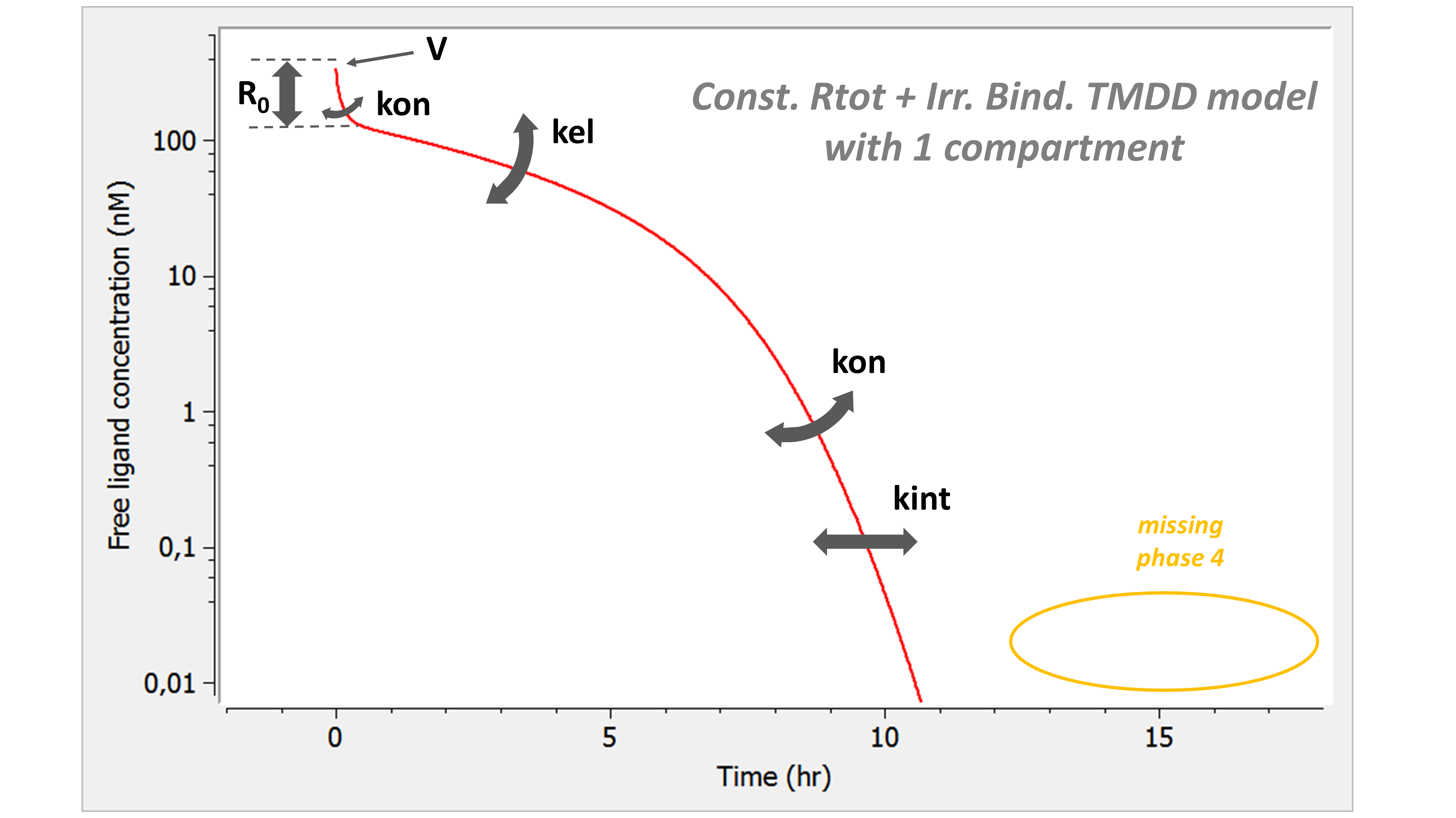
If one looks only at the free ligand concentration, this model is similar to the irreversible binding model. However it has one parameter less. Note that the phase 4 is missing.
Model with 2 compartments
If a second compartment is added, the shape is modified in the following way. Note that kon has been chosen large (very steep phase 1), to better focus on phase 2, where k12 and k21 have their main effect.
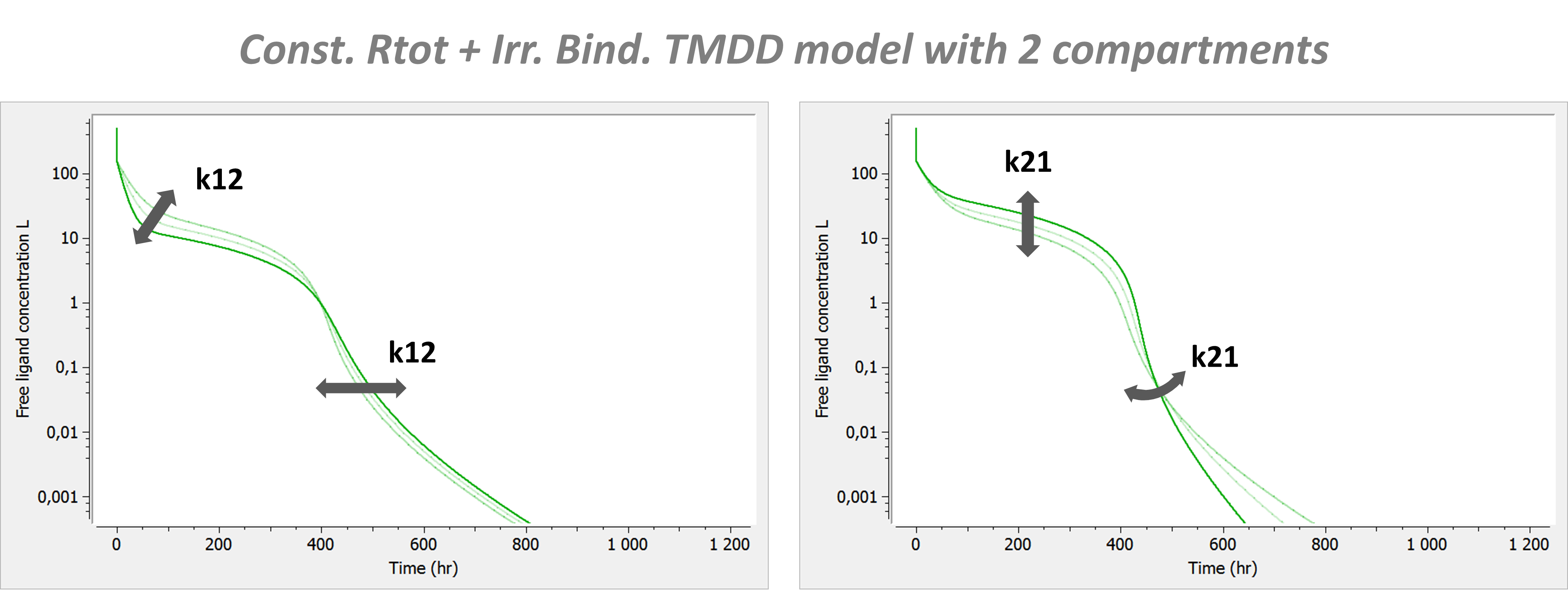
The introduction of a second compartment permits to recover a phase 4. Its flexibility is limited and linked to the effect of parameters k12 and k21 on phase 2.
Click here to go back to main TMDD page.
Detailed description of all the models
8.5.6.Wagner TMDD model
We here present the system of equation corresponding to the Wagner TMDD model, as well as the model behavior.
Equations
The constant Rtot, QSS/QE and irreversible binding approximations may still be overparametrized. A further simplification can be made and is called the Wagner model. It has initially been described in Biopharmaceutics and relevant pharmacokinetics by Wagner. The Wagner model can be derived from the QE/QSS approximation assuming in addition that the total receptor pool is constant (i.e 


Two formulations are possible, either using the free ligand concentration L or using the total ligand concentration Ltot. To our knowledge, the formulation using L is always presented:
}{V} - k_{\textrm{el}} \: L - \frac{R_0k_{\textrm{int}}L}{K_D+L} }{1+\frac{R_0K_D}{(K_D+L)^2}}")
with L the concentration of the ligand in plasma. V is the volume of the central compartment for the ligand, kel the linear elimination rate for the ligand, KD the dissociation constant, R0 the initial receptor concentration, and kint the degradation rate of the complex. In(t) represents the input function, corresponding to the input rate (amount per unit time) of the ligand into the central compartment due to the ligand administration.
If the system is derived from the QSS approximation, then KD is replaced by KSS. If it is derived from the irreversible model, then KD is replaced by 
This formulation presents a disadvantage: in case of a bolus administration, the initial free ligand concentration cannot be assumed to be 
however, the situation becomes more complicated for subsequent doses, where Rtot(t) must be used instead of Rtot(t=0)=R0.
![L(t=0)=\frac{1}{2}\left[ (\frac{D}{V}-R_0-K_{D})+\sqrt{(\frac{D}{V}-R_0-K_{D})^2+4K_{D}\frac{D}{V}}\right]](http://s0.wp.com/latex.php?latex=L%28t%3D0%29%3D%5Cfrac%7B1%7D%7B2%7D%5Cleft%5B+%28%5Cfrac%7BD%7D%7BV%7D-R_0-K_%7BD%7D%29%2B%5Csqrt%7B%28%5Cfrac%7BD%7D%7BV%7D-R_0-K_%7BD%7D%29%5E2%2B4K_%7BD%7D%5Cfrac%7BD%7D%7BV%7D%7D%5Cright%5D+&bg=ffffff&fg=000&s=0.5 "L(t=0)=\frac{1}{2}\left[ (\frac{D}{V}-R_0-K_{D})+\sqrt{(\frac{D}{V}-R_0-K_{D})^2+4K_{D}\frac{D}{V}}\right]")
We thus propose to use instead the formulation in Ltot (total ligand concentration):
![\begin{array}{ccl} \dfrac{dL_{\textrm{tot}}}{dt} &=& \dfrac{\textrm{In}(t)}{V} - k_{\textrm{int}} \: L_{\textrm{tot}} - (k_{\textrm{el}}-k_{\textrm{int}})L \\ L&=&\frac{1}{2}\left[ (L_{\textrm{tot}}-R_0-K_D)+\sqrt{(L_{\textrm{tot}}-R_0-K_D)^2+4K_DL_{\textrm{tot}}}\right] \end{array}](http://s0.wp.com/latex.php?latex=%5Cbegin%7Barray%7D%7Bccl%7D%C2%A0%5Cdfrac%7BdL_%7B%5Ctextrm%7Btot%7D%7D%7D%7Bdt%7D+%26%3D%26+%5Cdfrac%7B%5Ctextrm%7BIn%7D%28t%29%7D%7BV%7D+-+k_%7B%5Ctextrm%7Bint%7D%7D+%5C%3A%C2%A0L_%7B%5Ctextrm%7Btot%7D%7D+-+%28k_%7B%5Ctextrm%7Bel%7D%7D-k_%7B%5Ctextrm%7Bint%7D%7D%29L+%C2%A0+%5C%5C+L%26%3D%26%5Cfrac%7B1%7D%7B2%7D%5Cleft%5B+%28L_%7B%5Ctextrm%7Btot%7D%7D-R_0-K_D%29%2B%5Csqrt%7B%28L_%7B%5Ctextrm%7Btot%7D%7D-R_0-K_D%29%5E2%2B4K_DL_%7B%5Ctextrm%7Btot%7D%7D%7D%5Cright%5D+%5Cend%7Barray%7D&bg=ffffff&fg=000&s=0.5 "\begin{array}{ccl} \dfrac{dL_{\textrm{tot}}}{dt} &=& \dfrac{\textrm{In}(t)}{V} - k_{\textrm{int}} \: L_{\textrm{tot}} - (k_{\textrm{el}}-k_{\textrm{int}})L \\ L&=&\frac{1}{2}\left[ (L_{\textrm{tot}}-R_0-K_D)+\sqrt{(L_{\textrm{tot}}-R_0-K_D)^2+4K_DL_{\textrm{tot}}}\right] \end{array}")
The number of parameters is the same, and the system complexity also. P, R and Rtot can easily be calculated using 

")
=\frac{D}{V}=P(t=0)+L(t=0)")
With a second compartment, the system becomes:
![\begin{array}{ccl} \dfrac{dL_{\textrm{tot}}}{dt} &=& \dfrac{\textrm{In}(t)}{V} - k_{\textrm{int}} \: L_{\textrm{tot}} - (k_{\textrm{el}}-k_{\textrm{int}})L - k_{\textrm{12}}\:L + k_{\textrm{21}}\:A/V \\ \dfrac{dA}{dt} &=& k_{\textrm{12}}\:L\:V - k_{\textrm{21}}\:A \\ L&=&\frac{1}{2}\left[ (L_{\textrm{tot}}-R_0-K_D)+\sqrt{(L_{\textrm{tot}}-R_0-K_D)^2+4K_DL_{\textrm{tot}}}\right] \end{array}](http://s0.wp.com/latex.php?latex=%5Cbegin%7Barray%7D%7Bccl%7D%C2%A0%5Cdfrac%7BdL_%7B%5Ctextrm%7Btot%7D%7D%7D%7Bdt%7D+%26%3D%26+%5Cdfrac%7B%5Ctextrm%7BIn%7D%28t%29%7D%7BV%7D+-+k_%7B%5Ctextrm%7Bint%7D%7D+%5C%3A%C2%A0L_%7B%5Ctextrm%7Btot%7D%7D+-+%28k_%7B%5Ctextrm%7Bel%7D%7D-k_%7B%5Ctextrm%7Bint%7D%7D%29L+-+k_%7B%5Ctextrm%7B12%7D%7D%5C%3AL+%2B+k_%7B%5Ctextrm%7B21%7D%7D%5C%3AA%2FV+%5C%5C+%5Cdfrac%7BdA%7D%7Bdt%7D+%26%3D%26%C2%A0k_%7B%5Ctextrm%7B12%7D%7D%5C%3AL%5C%3AV+-+k_%7B%5Ctextrm%7B21%7D%7D%5C%3AA+%C2%A0%5C%5C+L%26%3D%26%5Cfrac%7B1%7D%7B2%7D%5Cleft%5B+%28L_%7B%5Ctextrm%7Btot%7D%7D-R_0-K_D%29%2B%5Csqrt%7B%28L_%7B%5Ctextrm%7Btot%7D%7D-R_0-K_D%29%5E2%2B4K_DL_%7B%5Ctextrm%7Btot%7D%7D%7D%5Cright%5D+%5Cend%7Barray%7D&bg=ffffff&fg=000&s=0.5 "\begin{array}{ccl} \dfrac{dL_{\textrm{tot}}}{dt} &=& \dfrac{\textrm{In}(t)}{V} - k_{\textrm{int}} \: L_{\textrm{tot}} - (k_{\textrm{el}}-k_{\textrm{int}})L - k_{\textrm{12}}\:L + k_{\textrm{21}}\:A/V \\ \dfrac{dA}{dt} &=& k_{\textrm{12}}\:L\:V - k_{\textrm{21}}\:A \\ L&=&\frac{1}{2}\left[ (L_{\textrm{tot}}-R_0-K_D)+\sqrt{(L_{\textrm{tot}}-R_0-K_D)^2+4K_DL_{\textrm{tot}}}\right] \end{array}")
with A the amount of ligand in peripheral tissues, k12 the rate of transfert from central to peripheral, and k21 the rate in the opposite direction.
Model properties
We investigate the influence of each parameter on the typical free ligand concentration-time shape for several dose amounts (bolus administration).

The summary picture is:
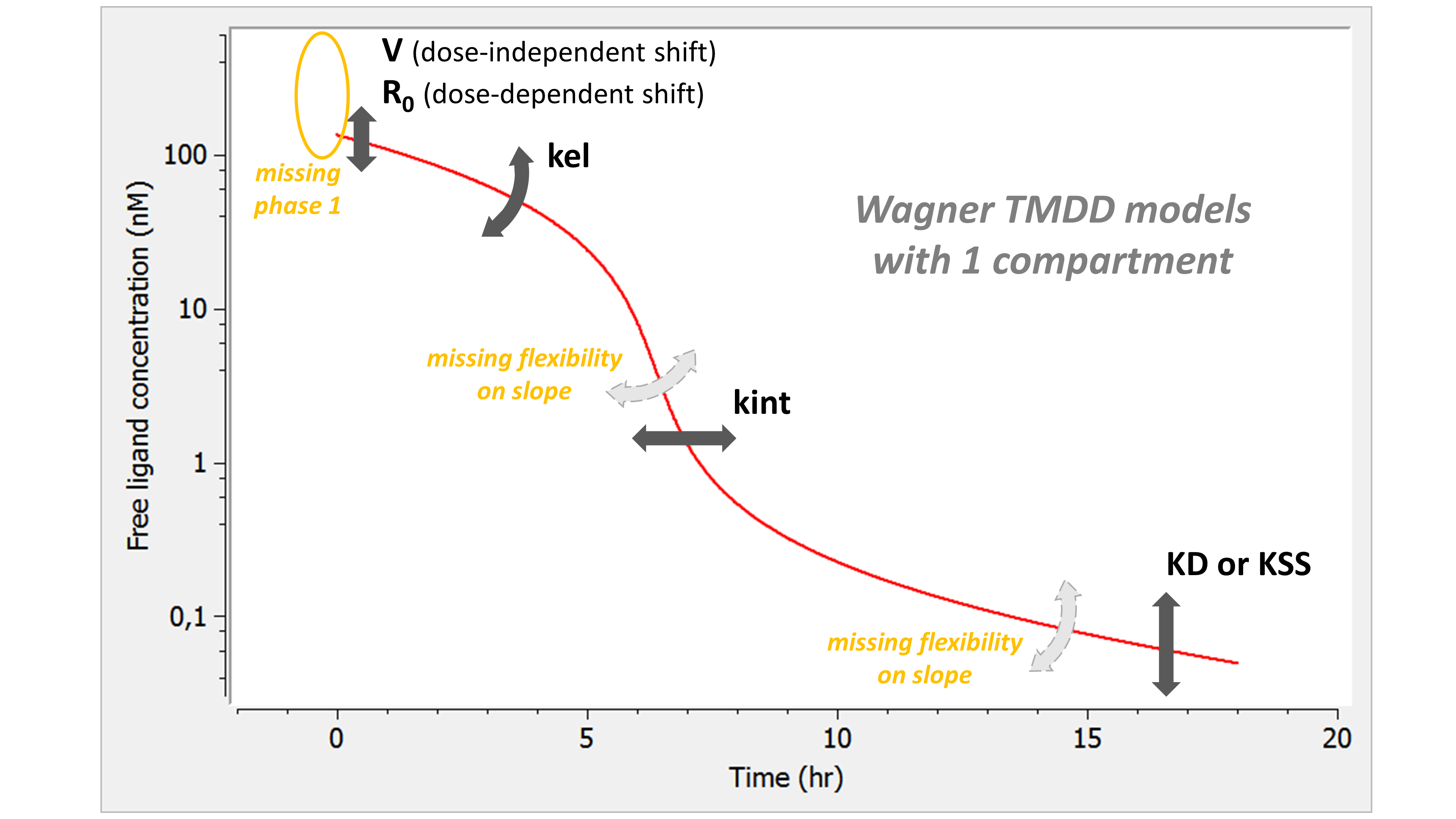
The Wagner model combines the assumptions of the QE (or QSS) model and those of the constant Rtot model. As for QE, the phase 1 is missing: the free concentration of ligand directly starts at the equilibrium concentration. In addition, the lack of kon passes on the lack of flexibility in the slope of phase 3. As for the constant Rtot model, we also have a lack of flexibility on the slope of phase 4.
Model with 2 compartments
If a second compartment is added, the shape is modified in the following way.
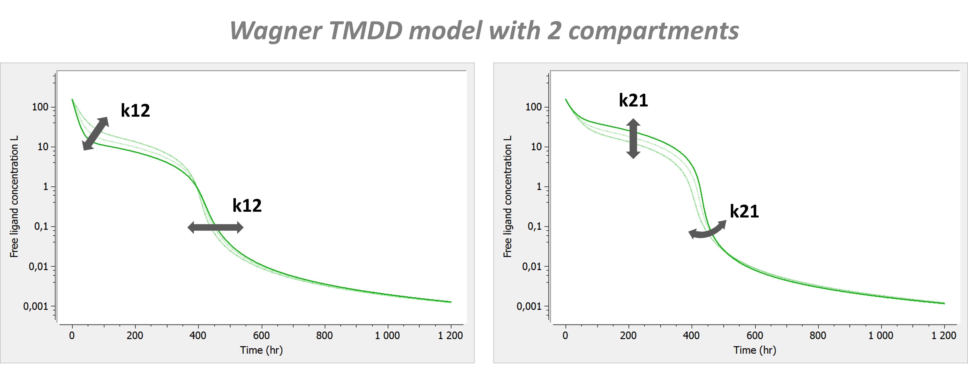
Click here to go back to main TMDD page.
Detailed description of all the models
8.5.7.Michaelis-Menten (MM) TMDD model
We here present the system of equation corresponding to the Michaelis-Menten (MM) TMDD model, as well as the model behavior.
Equations
The MM TMDD model has been proposed in Gibiansky et al. (2008), JPP 35(5). It is a further simplification of the Wagner model, assuming that ^2}\ll1")


}{V} - k_{\textrm{el}} \: L - \dfrac{V_m\:L}{K_D+L}")
with L the concentration of the ligand in plasma. V is the volume of the central compartment for the ligand, kel the linear elimination rate for the ligand, Vm the maximal velocity of the non-linear elimination and Km the Michaelis-Menten constant of the non-linear elimination. In(t) represents the input function, corresponding to the input rate (amount per unit time) of the ligand into the central compartment due to the ligand administration.
With a second compartment, the model becomes:
}{V} - k_{\textrm{el}} \: L - \dfrac{V_m\:L}{K_D+L} - k_{\textrm{12}}\:L + k_{\textrm{21}}\:A/V \\ \dfrac{dA}{dt} &=& k_{\textrm{12}}\:L\:V - k_{\textrm{21}}\:A \end{array}")
with A the amount of ligand in peripheral tissues, k12 the rate of transfert from central to peripheral, and k21 the rate in the opposite direction.
The MM model can also be derived from the “irreversible + constant Rtot” model, assuming a quasi state-steady on P (i.e -k_{\textrm{int}}P=0")
^2}\ll1")

In principle, a dose correction must also be applied in case of bolus administration, to split the incoming drug amount into free and bound ligand. However, the dose correction requires the use of one additional parameter, which would cancel out the advantages of the MM model compared to the Wagner or “constant Rtot + irreversible binding” models. Similarly, the concentrations of P, R, Rtot and Ltot could be calculated from the concentration of L, but this would require to use of R0 as additional parameter. The MM model with 4 parameters (6 if 2 compartments) is thus applicable only if the only measured species is the free ligand.
Model properties
We investigate the influence of each parameter on the typical free ligand concentration-time shape for several dose amounts (bolus administration).
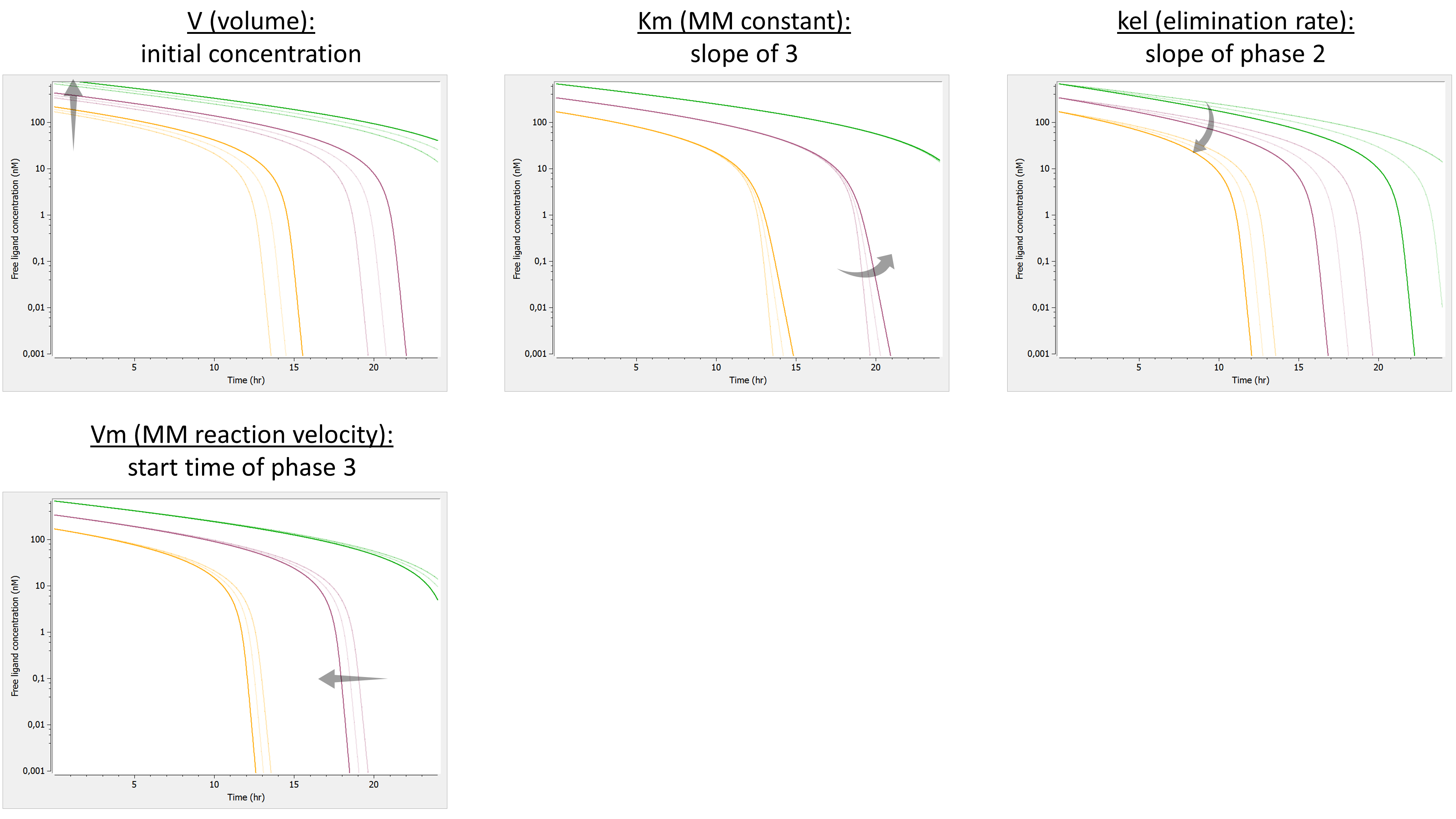
The summary picture is:
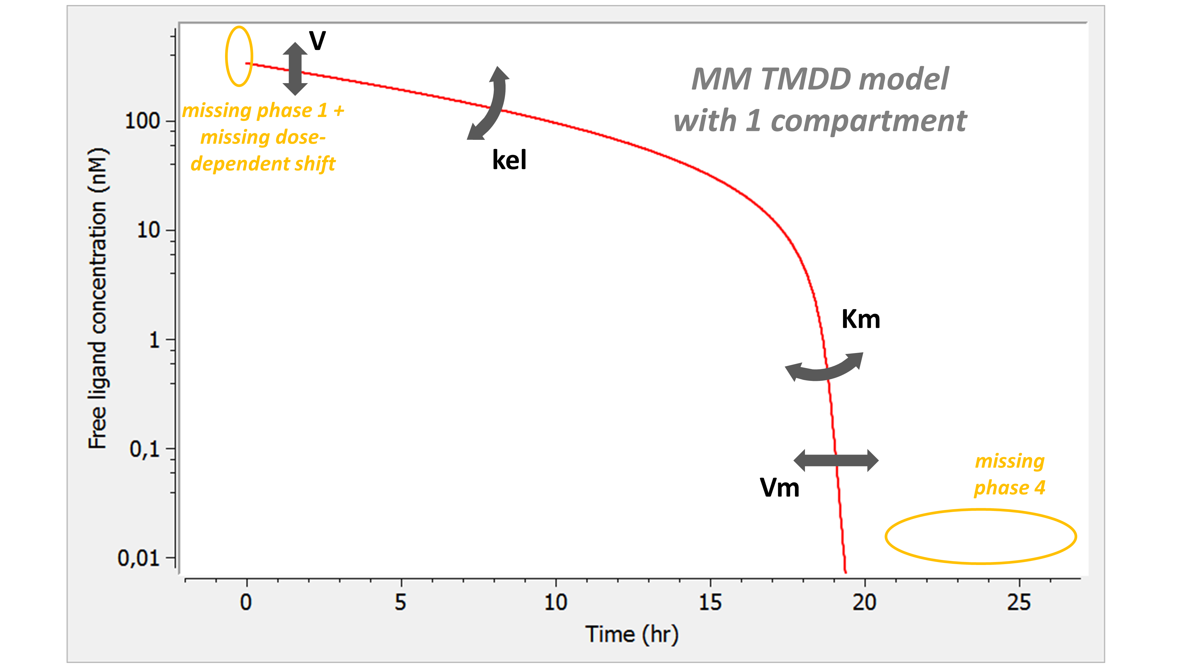
The MM model with one compartment does not capture phase 1 and phase 4. In addition, the dose-dependent shift of the initial concentration is missing: the free ligand concentration starts at the concentration obtained by dividing the dose amount by the volume, as if the ligand would not bind to the receptor. If the amount of administrated ligand is large compared to the amount of free receptor, this assumption is reasonable.
Model with 2 compartments
The MM model is often used with a second compartment. In this case the shape is modified in the following way:
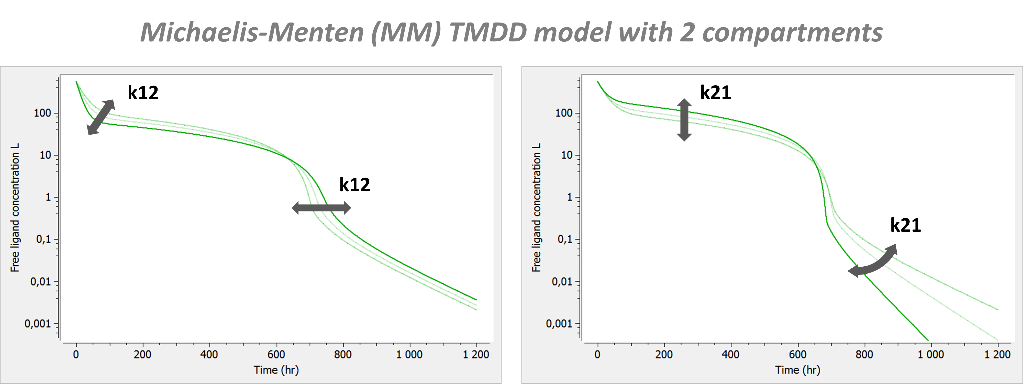
The introduction of a second compartment permits to recover a phase 4. Its flexibility is limited and linked to the effect of parameters k12 and k21 on phase 2.
Click here to go back to main TMDD page.
Detailed description of all the models
8.5.8.Guidelines to choose a TMDD model
The choice of a model is often not trivial. Because the data may not be sufficient to identify all the parameters of the full model, the parameter estimation process using the full model may not only lead to parameter estimates with large uncertainty but also fail to converge. This page gives guidelines to help the modeler to choose an appropriate TMDD model for his data set. The necessity of using simplified TMDD models is commonly the consequence of a limited data set and should not hide the fact that the reality may be more complex than the model.
In addition to using the TMDD approximation models (which are derived using assumptions on the parameter values), it is also possible to fix the unidentifiable parameter values, for instance using prior knowledge and typical values, while keeping the full TMDD model structure.
|
|
When to use a TMDD model
Several aspects can guide the choice of using a TMDD model.
First the type of molecule: biologics such as monoclonal anti-bodies, cytokines, growth factors, fusion proteins, antibody-small molecule drug conjugates or hormones are likely to display TMDD kinetics, at least in a certain concentration range. Notice that even if the biologic is eliminated via a TMDD mechanism, the typical TMDD behavior may not be observable due to too high or too low doses. In this case, a TMDD model will probably be over-parameterized. On the opposite, TMDD models should not be restricted to biologics as small molecules can also display TMDD kinetics (Guohua An (2017) J Clin Pharm 57(2)).
Second, the results of a non-compartmental analysis (NCA) can hint at TMDD kinetics if the apparent volume of distribution or the total clearance vary between the first dose and subsequent doses or for different dose amounts (Levy (1994), Clin Pharm Ther 56(3)).
Third, the shapes of the concentration-time curves is a key aspect. It will help to detect a TMDD behavior but also to choose the appropriate TMDD model among the several approximations possible.
How to choose a first model
Using prior information
The order of magnitude for some parameters might have been measured directly, for instance with in vitro experiments (e.g Biacore experiments, which usually provide kon and koff). This information can be used to choose an appropriate approximation:
- evidence of fast binding to receptor (high kon and koff) => QE, Wagner, MM
The influence of the kon parameter on the concentration-time curve is depicted below using Mlxplore, for typical parameter values. When kon is large, the initial drop of concentration due to the binding of the drug to the target is so fast that no data has been recorded in this part of the curve, therefore preventing a reliable estimation of kon. In this case, as can be seen on the right, the QE approximation gives the same concentration-time curve as the full model, except for the initial drop (phase 1).
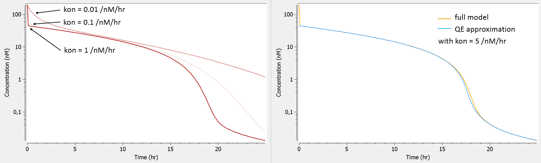 test
test - evidence of irreversible binding to receptor (very low dissociation constant KD) => IB, “const. Rtot + IB”, MM
The dissociation constant KD controls the height of the last phase (phase 4). When the binding affinity is very strong and thus the KD low, the last phase of the concentration-time curve is often below the LOQ and cannot be measured. In that case it is not possible to estimate KD and one can assume that the binding is irreversible. As can be seen on the left panel, the full model and the IB approximation model will differ in a part of the curve in which anyway no data had been recorded.
 test
test - evidence of similar rates for the elimination of free and bound receptor (kdeg and kint) => constant Rtot, Wagner, “const. Rtot + IB”, MM
In the plot below (left), we show the total concentration of receptor. When kint is larger than kdeg, the total receptor concentration will decrease after the ligand administration. Indeed, part of the receptor is then bound to the ligand and the complex is eliminated faster than the free receptor (kint>kdeg). Is is often the case in practice, as the binding of the ligand promotes the internalization of the receptor. On the opposite, when kint<kdeg, the total receptor concentration increases. Finally, when the complex internalization rate kint and the receptor degradation rate kdeg are very similar, the total receptor concentration is constant. The equation for the total receptor can then be dropped leading to a system with less parameters to estimate. When truly kint=kdeg, the constant Rtot model perfectly superimpose with the full model (right panel).
 test
test
Entities measured
Usually, in the case of a soluble target, the total ligand concentration (Ltot) is available, and sometimes the free ligand concentration (L) and/or the total target concentration (Rtot). For membrane-bound targets, usually the free ligand concentration (L) is available, and sometimes the target occupancy (TO) (see Gibiansky et al. PAGE 2011 Talk).
The following outputs are available for all models except the MM model: free ligand L, total ligand Ltot, free receptor R, total receptor Rtot, complex P, target occupancy TO and ratio of free receptor to baseline RR. Here are the restrictions in the model choice depending on the measured entities:
- only free ligand L measured => all models
- any other combination of measured entities => all models except MM
Shape of measured concentrations
As can be seen in the overview figure, the different approximations lead to different typical concentration shapes. As a consequence, the shape of the measured concentrations is a key element to choose an appropriate model. Two situations are particularly common: first, if the binding of the drug to the target is fast, phase 1 will be very short (in time) and measurements may only start after phase 1. In this case, the parameters related to the binding (especially kon) will not be identifiable and one can assume rapid-binding. Second, it may be that phase 4 appears at very low concentrations that are below the limit of quantification (LOQ). This may happen if the dissociation constant KD is small, i.e if the binding is almost irreversible.
- phase 1 not observable due to too rapid binding => QE, Wagner, MM
- phase 4 not observable because below LOQ => IB, “const. Rtot + IB”, MM
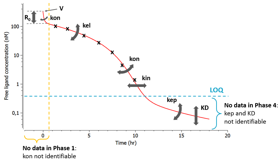
Range of doses
The initial receptor concentration R0 and the volume of the central compartment V have a similar influence on the ligand concentration-time curve, except that the shift induced by a volume change is dose-independent (same shift for all doses), while that induced by a change in R0 is dose-dependent (larger shift for small doses). If the tested doses do not range over a sufficient range, R0 may be difficult to identify. In this case the MM model may be a good approximation. If the MM model is not possible or insufficient, it is also possible to fix the value of R0.
The plots below show the concentration-time profile for different initial receptor concentrations (related to the receptor production and degradation rates via 
- C0>>R0: When the initial drug concentration (calculated as Dose/V) is small compared to the initial reception concentration, we recover the low dose case presented above, where only phase 1 and phase 4 can be seen.
- C0≈R0: When the initial ligand and receptor concentrations are of the same order of magnitude, the typical TMDD concentration-time curve shape is observed. The initial drop appears clearly and is dose-dependent. If several doses are tested, R0 (i.e kdeg) is likely to be identifiable.
- C0<<R0: When the initial drug concentration is much larger than the initial receptor concentration (which is often the case), the initial drop due to binding to the receptor is small on the scale of the ligand concentration and probably hard to quantify in the presence of measurement noise. In this case, the parameter R0 (or kdeg using the usual parameterization) which influences the height of the initial drop is usually not identifiable.
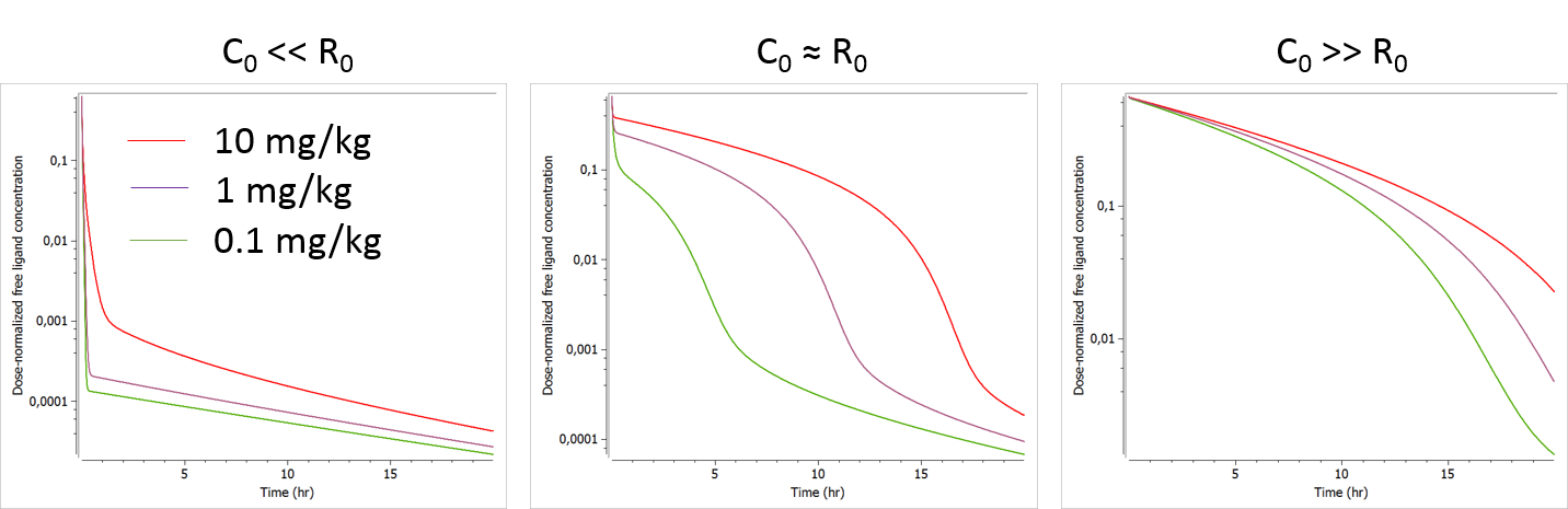
Improving the model
Bottom-up versus top-down approaches
A top-down approach to find an appropriate TMDD model has been proposed in Gibiansky et al. (2008), JPP 35(5). The procedure is the following: (i) fit the data with the full TMDD model, (ii) use the estimated parameters to simulate typical concentration-time curves with the full model and the approximations, (iii) if the simulations using a approximation are equivalent to the simulations with the full model, the approximation should be used. The strong disadvantage of this method is that the fitting of the full model may not converge, or give very uncertain estimates that are not informative and not reliable for simulations.
On the opposite, in a bottom-up approach, simpler models are tested first and progressively complexified if mis-specifications are detected in the diagnostic plots. Depending on the prior information, the first tested model can be any typical PK or TMDD model, and the diagnostic plots can help improving the model by removing one or several assumptions, in one or several steps. We recommend to use the bottom-up approach.
test
Examples of diagnostics
- Residuals (population weighted residuals, individual weighted residuals or normalized prediction distribution errors versus time or predictions): residuals plots help to detect if the model performs poorly for some specific times ranges or concentration ranges. Stratifying by dose group also permits to detect dose-dependent trends. An example is given below. The trend in the residuals indicates a model mis-specification. In this case a more complex model (with more parameters and thus more flexibility) can be tried.
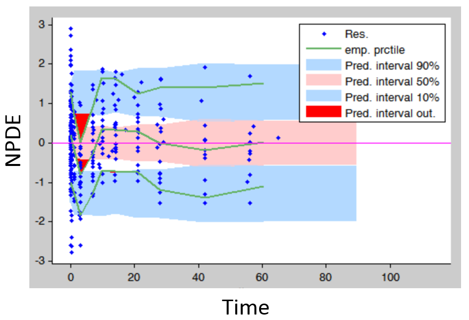
- Covariates: plotting the distribution of parameter values (or of random effects) for the different dose groups (which needs to be considered as a categorical covariate) allows to detect dose-dependent trends that indicate a model mis-specification. In the figure below (left), the individual parameters distribution of Vm is stratified by dose and shows a significant trend with increasing doses. This indicates that a more complex model is needed.
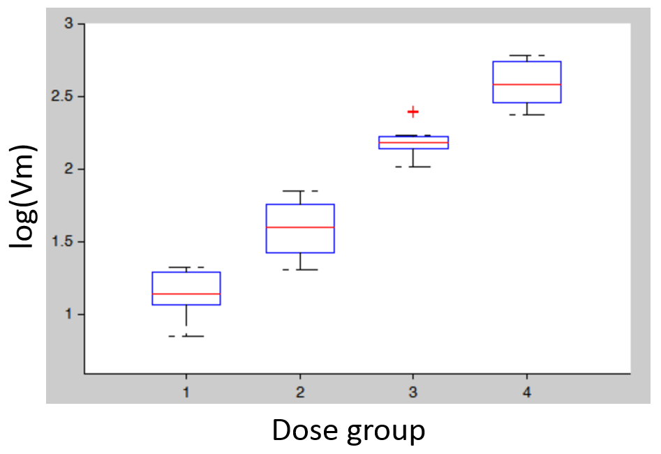
- Non-convergence of SAEM: if the fixed effect estimates is unstable and/or the omega value representing the standard deviation of the random effects converges to a very high value (see example below), the model is probably over-parameterized. Several options are possible to reduce the model complexity: (i) remove the inter-individual variability on this parameter, (ii) fix the value of the parameter, (iii) choose a model with less parameters.
- High condition number: the condition number is the ratio of the largest eigenvalue of the correlation matrix over the smallest value. High condition numbers hint at high correlations between parameters and thus model over-parameterizations. As a rule of thumb, condition numbers below 10 are ok, between 10 and 100 the model can be questionable, and above 100 the model is likely to be over-parameterized. In the example below, the high condition number probably reflects the high correlation between kdeg (kout) and KD. When the Monolix project is exported to Mlxplore using the last estimated parameters, one indeed clearly see that the influence of kdeg and KD on the concentration-time curve is the same. It will therefore not be possible to identify both. In this case, options are: (i) fix the value of one of the two parameters, or (ii) choose a model with less parameters.
 test
test - High r.s.e values: the r.s.e values indicate how uncertain the parameter estimate is. A high uncertainty may be the result of the parameter being unidentifiable because of lacking data. If a fixed parameter has a high r.s.e, one can try to either remove the IIV on this parameter, or fix this parameter value or try a model with less parameters. When an omega has a high r.s.e, one can try to remove the IIV on this parameter.

Conclusion
- Visualize and explore the data before starting the modeling.
- Have in mind how the parameters influence the curves. It is possible to check the influence for specific parameter sets with Mlxplore.
- Use the graphics to diagnose the model.
- Try several models, the librairie makes it easy.
- Consider several levels of flexibility:
- different model approximations, and 1 or 2 compartments
- parameters estimated or fixed
- parameters with or without inter-individual variability
- Keep in mind the ultimate modeling goal.
8.6.Tumor growth inhibition (TGI) library
A wide range of ODEs models for tumour growth (TG) and tumour growth inhibition (TGI) is available in the literature and correspond to different hypotheses on the tumor or treatment dynamics. In the absence of detailed biological knowledge, selecting the most appropriate model is a challenge. In MonolixSuite2020, we provide a modular TG/TGI model library that combines sets of frequently used basic models and possible additional features. This library permits to easily test and combine different hypotheses for the tumor growth kinetics and effect of a treatment, allowing to fit a large variety of tumor size data.
When available, analytical solutions are used.
Tumor growth models
Initial tumor size
The initial tumour size TS0 can be either be:
- a parameter to estimate,
- a regressor to read from the dataset.
It has to be noted that the time corresponding to the initial tumour size is not necessarily 0. It is the case for models implemented with an analytical solution, but for models implemented with an ODE system it corresponds to the initial integration time. This time is not fixed for most models from this library, which means that it is by default the first dose or observation time in the data set, and can vary between individuals. If one wishes to fix the initial integration time for all individuals, one can uncomment the line “t_0=0” in the model to fix the initial integration time at 0, and modify the line to choose another initial time, which must necessarily be before any dose or observation in the data set. Thus only models implemented with an analytical solution can capture observations at prior times than the time for TS0.
Kinetics of tumor growth
After a growing phase, tumors experience a saturation due to limits of nutrient supply. However, this saturation property is often never measured in patients in practice because the host dies in the majority of cases before this saturation phase begins. Also in preclinics, the experiments have to be canceled if a specific tumor size is reached due to ethical reasons. Thus, tumor growth models may be divided into two broad categories: those which are able to capture the saturation as the tumor grows (achieved by the introduction a carrying capacity or a spontaneous decay component) and those which do not.

-
Models without saturation
-
Linear
-
The linear tumor growth assumes a constant zero-order growth rate.
| ODE system | Analytical solution |  |
|
$$ \frac{dTS}{dt} = kgl $$ $$ TS(t_0)=TS0 $$ |
$$ TS=kgl*t+TS0 $$ |
-
-
Quadratic
-
The quadratric tumor growth combines linear and quadratic growth rates. Because time is involved in this model, the initial time is fixed to 0 in corresponding library models.
| ODE system | Analytical solution | 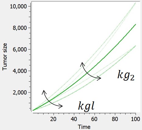 |
|
$$ \frac{dTS}{dt} = kgl+2*kg2*t $$ $$ TS(t_0)=TS0 $$ |
$$ TS=kgl*t+kg2*t^2+TS0 $$ |
-
-
Exponential
-
The exponential growth assumes the growth rate of a tumor is proportional to tumor burden (first-order growth).
| ODE system | Analytical solution |  |
|
$$ \frac{dTS}{dt} = kge*TS $$ $$ TS(t_0)=TS0 $$ undefined |
$$ TS=TS0*e^{kge*t} $$ |
-
-
Power law
-
If 0 < gamma < 1, the power law model (also named generalized exponential) provides a description in terms of a geometrical feature of the proliferative tissue: the growth rate is proportional to the number of proliferative cells as a fraction of the full tumor volume. The case gamma=1 corresponds to proliferative cells uniformly distributed within the tumor and leads to exponential growth. The case gamma=2/3 represents a proliferative rim limited to the surface of the tumor, where the tumor radius grows linearly in time.
| ODE system | Analytical solution | 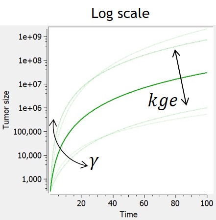 |
|
$$ \frac{dTS}{dt} = kge*TS^\gamma $$ $$ TS(t_0)=TS0 $$ |
$$ TS=(kge*(1-\gamma)*t+TS0^{1-\gamma})^{\frac{1}{1-\gamma}} $$ |
-
-
Exponential-linear
-
Experimental data of tumor growth in untreated xenograft mice suggest that tumor growth dynamics follow two distinctively different phases of growth: an initial exponential growth, followed by a linear growth phase. Biologically, this is due to the fact that the growth of the tumor is almost unlimited at first, but that as the nutrients go scarce, its growth is then necessarily restricted.
The simple exponential-linear model captures this with a transition between an exponential (first-order) growth to a linear (zero-order) growth. The transition time is computed to ensure that the solution is continuously differentiable, but this is possible only if the model is not combined with any treatment effect or additional features. In that case, the transition time corresponds to TS = kgl/kge.
In the library, the exponential-linear model is provided with its analytical solution and can not be combined to any treatment effect or additional features.
| ODE system | Analytical solution | 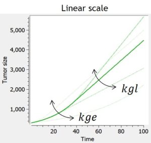 |
|
$$ \frac{dTS}{dt} = kge*TS, t\le\tau$$ $$ \frac{dTS}{dt} = kgl, t\ge\tau$$ $$ TS(t_0)=TS0 $$ $$\tau = \frac{1}{kge}ln(\frac{kgl}{kg*TS0})$$ |
$$ TS=TS0*e^{kge*t}, t\le\tau $$
$$ TS=kgl*(t-\tau)+TS0*e^{kge*\tau}, t\ge\tau $$ $$\tau = \frac{1}{kge}ln(\frac{kgl}{kg*TS0})$$ |
-
-
Simeoni
-
The Simeoni model approximates the exponential-linear model with a single differential equation. The power term is fixed to 20 to allow the system to pass from the first-order to the zero-order growth sharply enough, as in the original system. With this value, the growth rate is approximated by kge*TS when TS is smaller than kgl/kge, and by kgl when TS is larger than kgl/kge. The advantage of the Simeoni model over the exponential-linear model is that it is differentiable even when combined with any type of treatment effect.
When used in combination with the description of non-proliferating subpopulations of cells (transit compartments with cell distribution, or two populations model), with TS the size of the proliferating subpopulation, the growth function is slowed down by the factor TS/TotalTS only when the tumor is in its linear growth phase, but not in the exponential growth phase.
| ODE system | Reference | 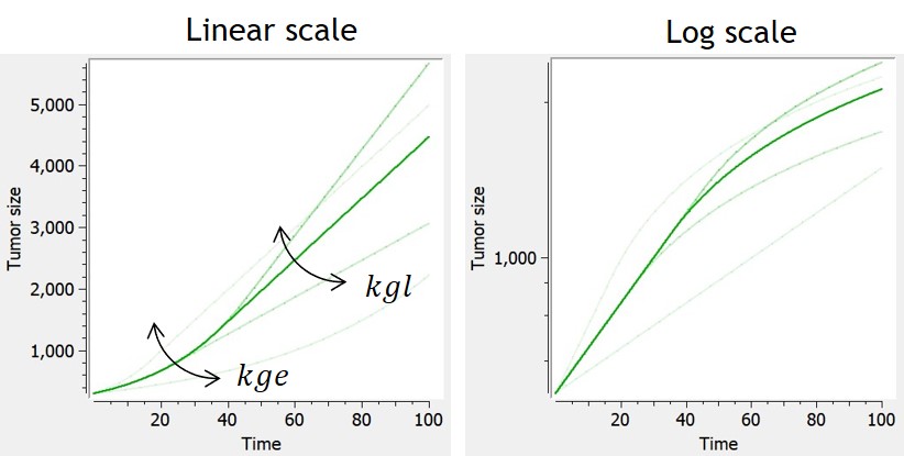 |
|
$$ \frac{dTS}{dt} = \frac{kge*TS}{(1+(\frac{kge}{kgl}*TS)^\psi)^(\frac{1}{\psi}} $$ $$ TS(t_0)=TS0 $$ |
Simeoni et al. (2004). |
-
-
Koch
-
Similarly to the exponential-linear and Simeoni models, the Koch tumor growth model is a nonlinear growth function that follows an initial exponential growth followed by a linear growth phase. Its particularity is a smooth transition between exponential and linear growth phase, rather than a rapid switch after a threshold reached for the time (exponential-linear) or tumor size (Simeoni).
When used in combination with the description of non-proliferating subpopulations of cells (transit compartments with cell distribution, or two populations model), with TS the size of the proliferating subpopulation, the growth function is slowed down by the factor TS/TotalTS.
| ODE system | Analytical solution | Reference | 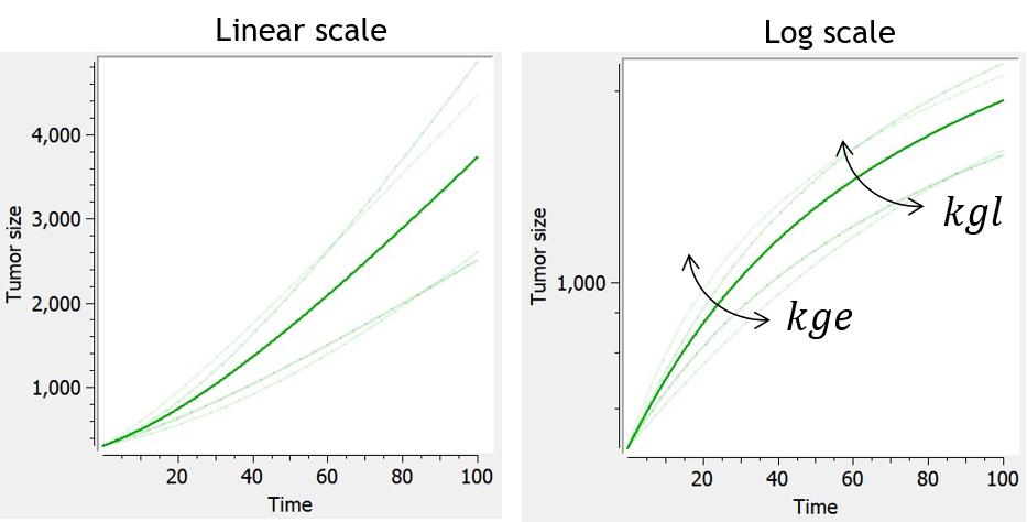 |
|
$$ \frac{dTS}{dt} = \frac{2kge*kgl*TS}{kgl+2kge*TS} $$ $$ TS(t_0)=TS0 $$ |
$$ TS=TS0e^{2kge(t+\frac{1}{kgl}(TS0-TS))} $$ | Koch et al. (2009) |
-
Models with saturation
-
Logistic
-
This model assumes an exponential growth rate which decelerates linearly with respect to the tumor size. This results in sigmoidal dynamics – with an initial exponential growth phase followed by a growth-saturated phase as the tumor reaches its carrying capacity (TSmax).
| ODE system | Analytical solution | 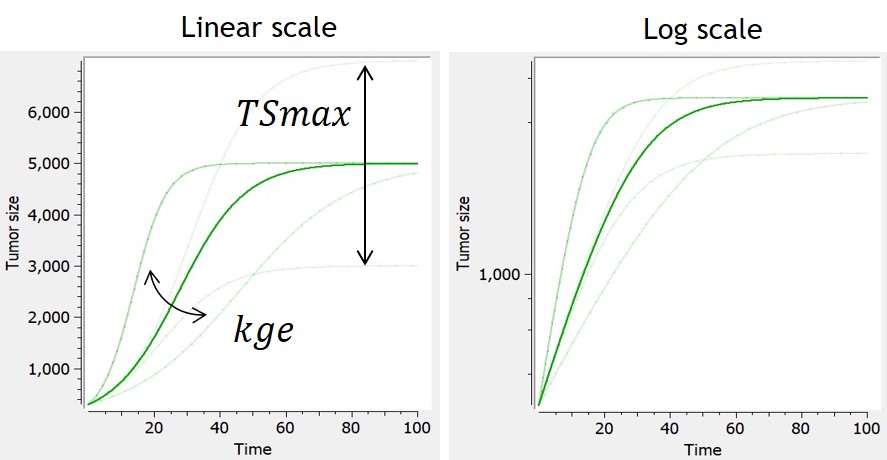 |
|
$$ \frac{dTS}{dt} = kge*TS(1-\frac{TS}{TSmax}) $$ $$ TS(t_0)=TS0 $$ |
$$ TS=\frac{TSmax*TS0}{TS0+(TSmax-TS0)*e^{-kge*t}} $$ |
-
-
Generalized logistic
-
In this model, tumor growth depends on tumor size with a generalized logistic function. It reduces to the logistic model if 

| ODE system | Analytical solution | 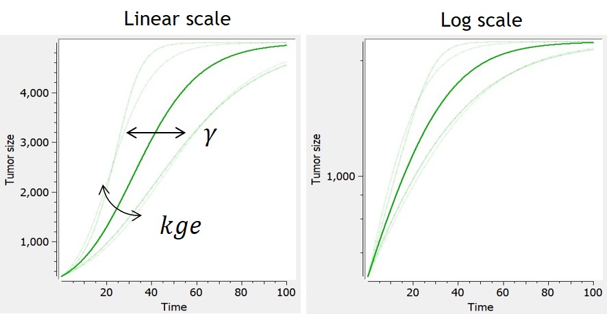 |
|
$$ \frac{dTS}{dt} = kge*TS(1-(\frac{TS}{TSmax})^{\gamma}) $$ $$ TS(t_0)=TS0 $$ |
$$ TS=\frac{TSmax*TS0}{(TS0^\gamma+(TSmax^\gamma-TS0^\gamma)*e^{-kge*\gamma*t})^{\frac{1}{\gamma}}} $$ |
-
-
Simeoni-logistic
-
In [Haddish-Berhane et al., 2013], a hybrid model derived from the Simeoni model is proposed, that combines exponential, linear and logistic growth.
| ODE system | Reference | 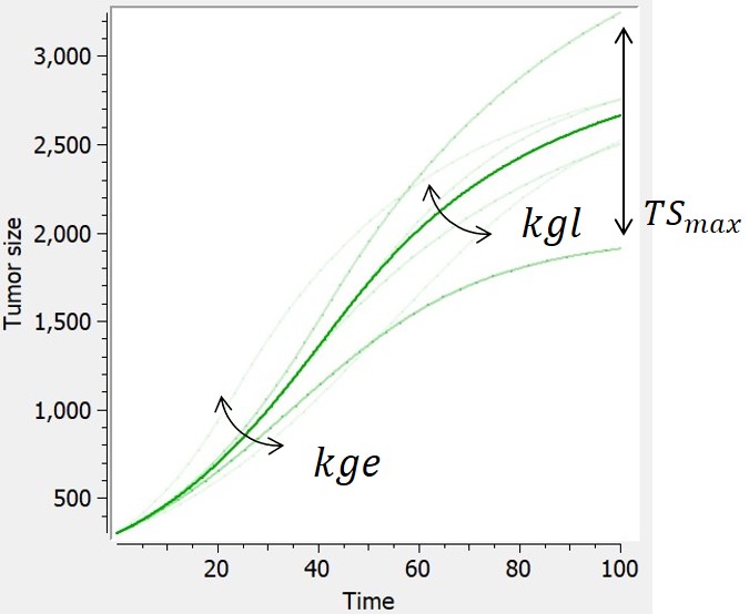 |
|
$$ \frac{dTS}{dt} = \frac{kge*TS*(1-\frac{TS}{TSmax})}{(1+(\frac{kge}{kgl}*TS)^\psi)^{\frac{1}{\psi}}} $$ $$ TS(t_0)=TS0 $$ |
Haddish-Berhane et al., 2013 |
-
-
Gompertz
-
The Gompertz model follows the observation of a deceleration of the growth rate over time, without any phase at which the growth rate remains constant. The volume converges asymptotically to ")
Several parameterizations can be used, and two are displayed on the table below. The first parameterization is the one implemented in the library, and the one for which the impacts of the parameters are the most separate and easiest to control. However, the carrying capacity TSmax can be difficult to estimate and can lack biological meaning if no clear tumor size saturation is seen. With the second parameterization, alpha and beta have an impact on the carrying capacity and on the growth rate, while TS0 also has an impact on the carrying capacity.
| ODE system | Analytical solution | |
|
$$ \frac{dTS}{dt} = TS*\beta*ln(\frac{TSmax}{TS}) $$ $$ TS(t_0)=TS0 $$ |
$$ TS=TSmax*e^{e^{-\beta*t}*ln(\frac{TS0}{TSmax})} $$ | 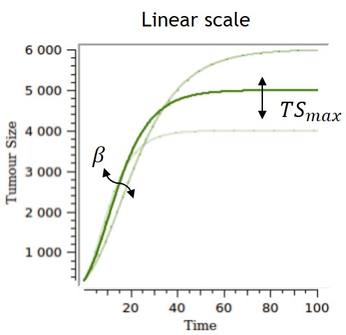 |
| $$ \frac{dTS}{dt} = \alpha*e^{-\beta*t}*TS $$
or, equivalently, $$ \frac{dTS}{dt} = (\alpha-\beta*ln(TS))TS $$ $$ TS(t_0)=TS0 $$ |
$$ TS=TSmax*e^{e^{-\beta*t}*ln(\frac{TS0}{TSmax})} $$ | 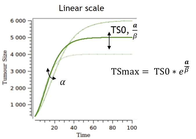 |
-
-
Exponential-Gompertz
-
An exponential-Gompertz model can also be considered, built upon the assumption that the tumor follows at first an exponential growth, and is then akin to a Gompertz model once the nutrients start to go scarce.
| ODE system | Refefence | 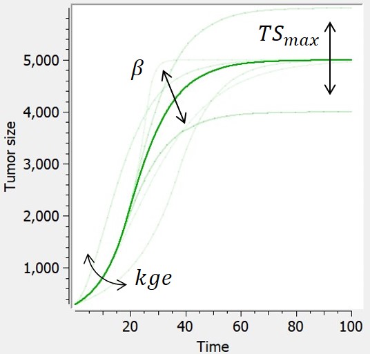 |
|
$$ \frac{dTS}{dt} = min(kge*TS,TS*\beta*ln(\frac{TSmax}{TS})) $$ $$ TS(t_0)=TS0 $$ |
Wheldon (1988) |
-
-
Von Bertalanffy
-
This model is based on balance equations of metabolic processes. The growth is limited with a loss term.
| ODE system | Analytical solution | Reference | 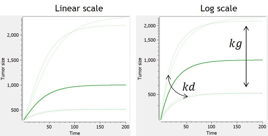 |
|
$$ \frac{dTS}{dt} = kg*TS^{2/3}-kd*TS $$ $$ TS(t_0)=TS0 $$ |
$$ TS= \left[ \frac{kg}{kd}+(TS0^{1/3}-\frac{kg}{kd})*e^{-1/3*kd*t} \right]^3 $$ | Von Bertalanffy, 1957 |
-
-
Generalized Von Bertalanffy
-
This is the generalized version of the Von Bertalanffy model. The von Bertalanffy model corresponds to the case gamma=⅔, where the growth is proportional to the surface of the tumor.
The loss term induces for some parameter values a saturation of the tumor, with ^{\frac{1}{1-\gamma}}")
When the Von Bertalanffy model (or generalized Von Bertalanffy model) is used in combination with a tumor inhibition model which makes use of the Norton Simon killing hypothesis, the treatment effect is only applied to the growth term of the model (and not to its decay term).
| ODE system | Analytical solution | Reference | 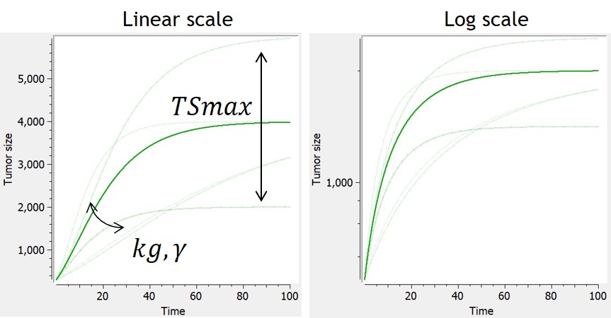 |
|
$$ \frac{dTS}{dt} = kg*TS^{\gamma}-kd*TS $$ $$ 0 \leq \gamma \leq 1 $$ $$ TS(t_0)=TS0 $$ |
$$ TS= \left[ \frac{kg}{kd}+(TS0^{1-\gamma}-\frac{kg}{kd})*e^{-(1-\gamma)*kd*t} \right]^\frac{1}{1-\gamma} $$ | Von Bertalanffy, 1957 |
Additional features
Additional features can be included to consider more complex tumor growth models:
-
Dynamic carrying capacity due to angiogenesis
The library includes, as an example, a module taken from Hahnfeldt et al,1999 that models the effect of angiogenesis as a dynamic carrying-capacity. When selecting the dynamic carrying-capacity module, TSmax is defined as an ODE variable instead of a constant parameter, with the following ODE:
| ODE | Reference | 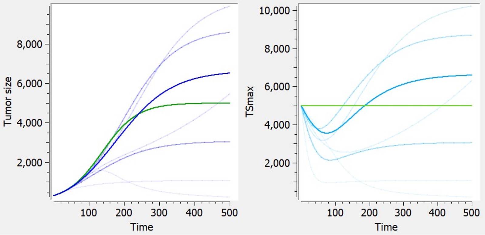 Examples of curves for tumor size (left) or carrying capacity (right) with diverse shapes, based on logistic tumor growth. Green: predictions without the additional feature (constant TSmax). Blue: with dynamic carrying capacity. Examples of curves for tumor size (left) or carrying capacity (right) with diverse shapes, based on logistic tumor growth. Green: predictions without the additional feature (constant TSmax). Blue: with dynamic carrying capacity. |
|
$$ \frac{dTS_{max}}{dt} = kp_v*TS -\kappa*TS_{max} – kd_{\nu}*TS*TS^{2/3} $$ |
Hahnfeldt et al,1999 |
-
Immune dynamics causing shrinkage or oscillations of tumor size
The library includes, as an example, a model of tumor-immune interactions with chemotherapy proposed by De Pillis et al. (2007), taking into account the control of the tumor growth by the immune system, and the weakening of the immune system as a side effect of chemotherapy. The model includes an additional ODE defining effector–immune cells:
| ODE system | Reference | 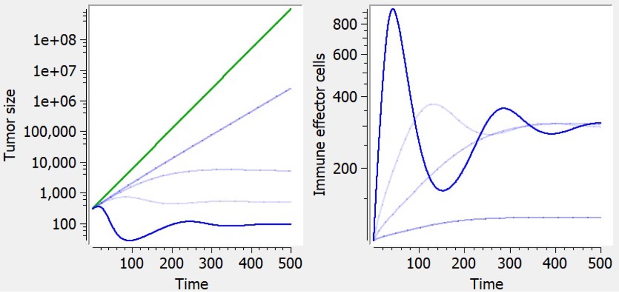 Examples of curves for tumor size (left) or effector immune cells (right) with diverse shapes, based on exponential tumor growth. Green: prediction without the additional feature (constant tumor growth). Blue: with immune dynamics. Examples of curves for tumor size (left) or effector immune cells (right) with diverse shapes, based on exponential tumor growth. Green: prediction without the additional feature (constant tumor growth). Blue: with immune dynamics. |
|
$$ \frac{dTS}{dt} = growth -ki*I*TS $$ |
De Pillis et al. (2007) |
More details on these additional features.
Treatment effect
Type of treatment
Flexible treatment definition is provided thanks to several possibilities:
- No treatment
This option corresponds to simple tumor growth models.
- PK model
Dosing information is encoded in the dataset, and the effect of the treatment is modeled via a simple PK model (one compartment, bolus administration, linear elimination) which can be easily adapted to a more complex model or to fix some parameters. The predicted concentration inhibits tumor size.
Note that in case of a high number of doses, it is preferable to approximate the exposure by a piecewise regressor or by a constant treatment, to reduce computation cost. Particularly when the dosing is daily and the disease lasts several years, modeling of the PK is not useful and very costly.
- Exposure as regressor
Values which describe the evolution of the treatment’s exposure/concentration with respect to time are already stored within the data set and are used within the TGI model under the variable EXPOSURE.
DATA FORMAT RESTRICTIONS: The values describing the treatment’s exposure with respect to time must be stored in a separate column of the data set labelled ‘REGRESSOR’.
- Treatment start at t=0
The tumour growth inhibition component is applied with a constant effect after t=0.
DATA FORMAT RESTRICTIONS: The data must be formatted as to have the treatment being added at time t=0 for all individuals. Measurements before that can make use of negative values for time. Note that in that case, the initial integration time (corresponding to the initial tumour size TS0) is the first measurement time and can vary between individuals.
- Treatment start time as regressor
The time at which the treatment is added is a variable named T in the model, which may vary between individual, and whose value is read from a regressor column in the data set. When time t<T, a simple tumour growth model is being implemented. After, a tumour growth inhibition component to the model is added.
DATA FORMAT RESTRICTIONS: The values for T must be stored within the data set in a separate column tagged as ‘REGRESSOR’.
- No treatment (0) vs treatment (1) regressor
A simple tumour growth model is being implemented if the variable Trt = 0. If Trt = 1, a tumour growth inhibition component to the model is added. Trt is read from a regressor column in the dataset.
DATA FORMAT RESTRICTIONS: A 0 – if the measurement was taken before or after treatment – or 1 – if it was taken during treatment – must be matched and stored within a separate column under the header ‘REGRESSOR’ for each of the measurements of the data set.
Killing hypothesis
There are two different most commonly used hypothesis relevant to the method of killing of any given treatment within the literature:
|
|
If the growth is exponential (
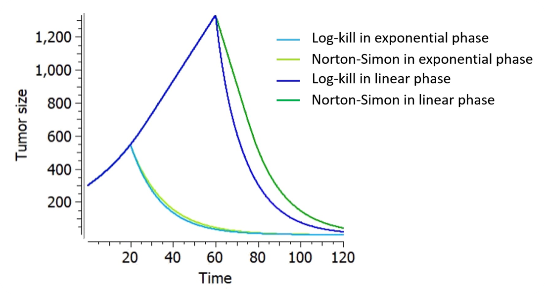
On the figure on the right for example, the tumor size follows an exponential-linear growth, a constant treatment effect is applied either in the exponential phase (at t=20) or in the linear phase (at t=60). The treatment kinetics is linear. The parameters are adapted such that 
It enfolds that under the Norton-Simon hypothesis the optimal treatment should deliver the most effective dose level of drug over as short a time as possible (high dose density), since tumors given less time to grow between treatments are more likely to be eradicated.
Dynamics of treatment effect
Five different exposure-dependent treatment kinetics which we found to be most common within the literature can be combined with both of these killing hypotheses.
Below are plots showing the curves resulting from the addition of these TGI models to an exponential TG model, with a punctual drug exposure resulting from a single dose which is absorbed at time 0 and then eliminated. On the first figure, a linear range of different dose amounts has been applied in order to exhibit the linear and non-linear relationships between exposure and treatment effect.

When the treatment exposure is not given, the treatment effect is constant.
Delay of treatment effect
Chemotherapeutic effects often appear days or weeks following drug exposure. To account for a more progressive tumour regression, a delay in either the treatment effect (i.e. signal distribution model) or cell death (i.e. cell distribution model) may be added via transit compartments.
-
Signal distribution model
Lobo and Balthasar (2002) applied to tumor growth the transit compartment model proposed by Sun & Jusko (1998) to characterize delayed drug effects that occur via a cascade or signal transduction. The operative rate function of tumor cells killing, K3, is related to K via a series of transit compartments (K1-K3). Tau refers to the mean transit time in each transit compartment. Although 4 transit compartments were used in Lobo and Balthasar (2002), the model implemented in our library has only 3 compartments for an easier comparison to the cell distribution model. It can be easily edited by the user to add more compartments if nedded.
-
Cell distribution model
The cell distribution model proposed in Simeoni et al., 2004 assumes that the anticancer treatment makes some cells non-proliferating. These cells pass through different stages (also called transit compartments), characterized by progressive degrees of damage, and, eventually, they die. Hence, the attacked tumor cells have a lifespan.
The number of stages of damage and the value of tau affect the shape of the distribution of the time-to-death of damaged tumor cells. The lifespan, or time-to-death, of the attacked tumor cells, is the mean transit time that it takes for the tumor cells, affected by the action of a drug, to go through the cascade of damaging events to cell death. For n transit compartments, the average lifespan is computed by Mtt = n*tau. This library includes an implementation of the model with three transit compartments, as in Simeoni et al., 2004.
When the model considers two populations of cancer cells in the tumor (sensitive/resistant), the treatment induces the transfer or both types of cells into the first transit compartment, with different rates.
Below are plots showing the curves resulting from the addition of both of these delays to a model making use of exponential TG component and a log-kill constant TGI component depending on constant treatment starting at time 30.
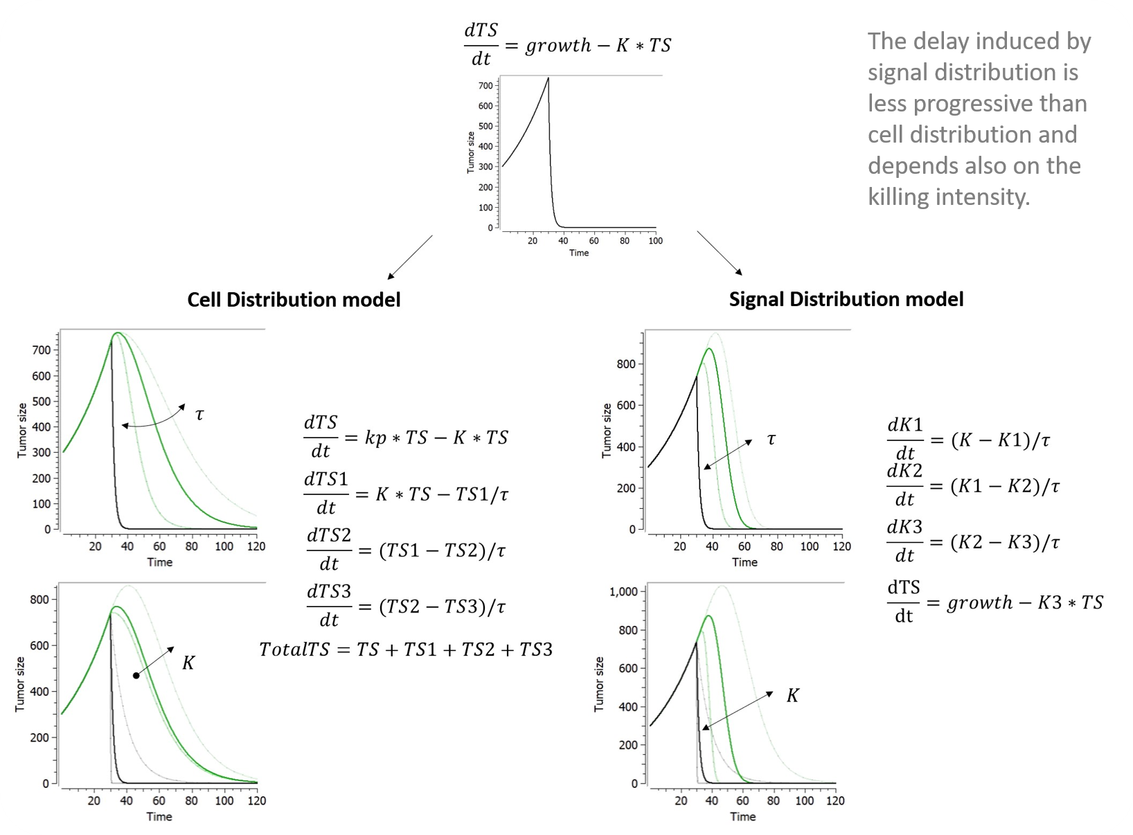
Emergence of resistance
A common feature of tumours is the emergence of treatment-resistance. This phenomena can be modelled in a variety of ways. Decrease in treatment efficacy can be simply added in a phenomenological approach. More mechanistic models try to represent the cell population in its heterogeneity, splitting it into at least two subpopulations: the proliferating and the quiescent cells.
In this library, we included two common methods used within the literature to achieve this:
-
Claret exponential
This simple phenomenological model accounts for the loss of drug-induced decay over time due to declining efficacy of the drug, which can be due to the emergence of resistance. It uses a single resistance parameter 
| Equation | Refefence | 
Figure for an exponential growth function and constant treatment effect starting at time t=0. |
|
$$ K’ = K*e^{-\lambda*t} $$ |
Claret et al. (2009) |
-
Resistant population
There are many models in the literature that apply variations of the same approach based on two tumor cell populations with different sensitivities, for example Hahnfeldt et al., 2003, Desmée et al., 2017, Lobo & Balthasar, 2002, Jusko, (1973). We have integrated in the library simple versions inspired by this principle, combined with different treatment effects: these models assumes that a fraction of the tumor is resistant to the treatment, thus being killed with a smaller rate than the sensitive part of the tumor. They use a parameter f as initial fraction of resistant tumour cells, and the number of parameters characterizing the treatment effect doubles to have population-specific effects.
| Equation | 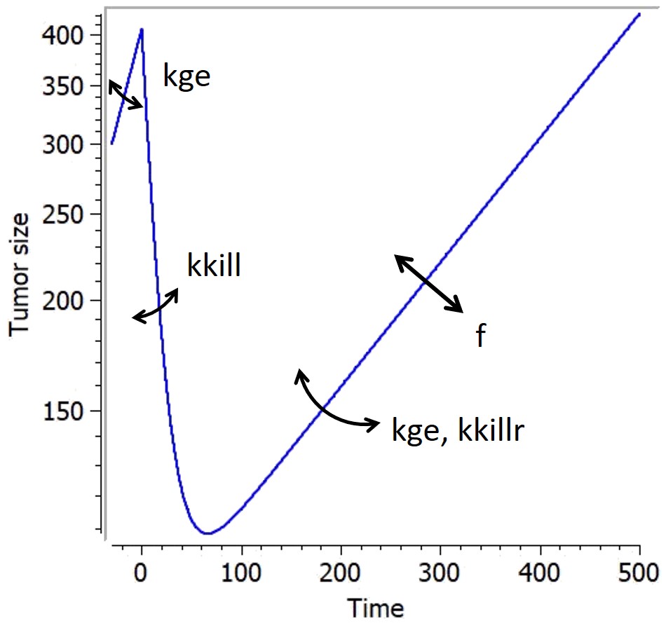
Figure for an exponential growth function and constant treatment effect starting at time t=0. |
| Log-killl hypothesis:
$$ \frac{dTS_s}{dt} = growth – TS_s*K_{TS_s}$$ $$ \frac{dTS_r}{dt} = growth – TS_r*K_{TS_r}$$ Norton-Simon hypothesis: $$ \frac{dTS_s}{dt} = growth * (1- K_{TS_s})$$ $$ \frac{dTS_r}{dt} = growth *(1-K_{TS_r})$$ Initial conditions: $$ TS_s(t_0)=TS0*(1-f) $$ $$ TS_r(t_0)=TS0*f $$ |
Below is a figure showing the curves resulting from the addition of these two resistance components to a model making use of exponential TG component and a log-kill linear TGI component, with a constant treatment effect starting at time 0.
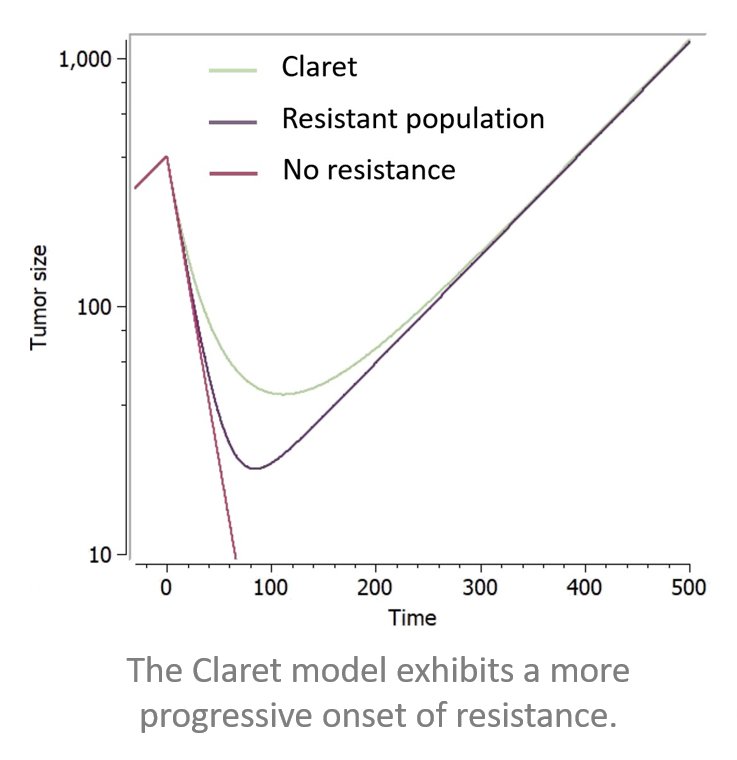
Effect of treatment on angiogenesis or immune dynamics
If more complexity was added to the TG model by means of modelling immune dynamics or a dynamic carrying capacity, it can be decided that these should also be influenced by the addition of a treatment.
-
Combination therapy with active inhibition of angiogenesis
Combination therapy is often used to maximise chances of tumour regression and minimise chances of treatment-resistant clones from emerging. As such, it may be wished to model the effect of an angiogenesis inhibitor, on top of the tumour inhibitor. This corresponds to an additional option named “Additional treatment effect” available in the library when both angiogenesis and a treatment effect are selected. In that case the ODE for TSmax becomes:
$$ \frac{dTS_{max}}{dt} = kp_v*TS -\kappa*TS_{max} – kd_{\nu}*TS*TS^{2/3} -e*TS_{max} $$
The treatment on angiogenesis is added as a second constant treatment (on top of the one selected earlier on). By choosing this additional option, it is assumed that no PK data is available for this second treatment and consequently, first-order kinetics are used to model the effect. Furthermore, the effect of the second treatment is assumed to follow a log-cell kill killing hypothesis.
-
Combination therapy with decay of immune cells
If the treatment added does not only target tumour cells but a more general cell population (such as chemotherapy), it may be relevant to include a killing term on the immune cell dynamics as well. This feature is available in the library if modelling of immune dynamics was selected during selection of tumour growth model. It consists in adding an extra decay constant to take into consideration the effect chemotherapy will have on immune cells. The equations then become:
$$ \frac{dI}{dt} = kp_i – kd_i*I + g*\frac{TS}{h+TS}*I -p*I*TS – K_i*I $$
where the killing term 
Shortcut models
Lastly, we found that some typical models within the literature. In order to ease access to these models, we created a shortcut tab which automatically leads one to the appropriate selections when applicable, or loads the dedicated model otherwise. In each case, the initial tumor size TS0 can be set as a parameter or as a regressor.
-
Claret exponential model
This model from Claret et al., 2009 corresponds to the following choices in the library:
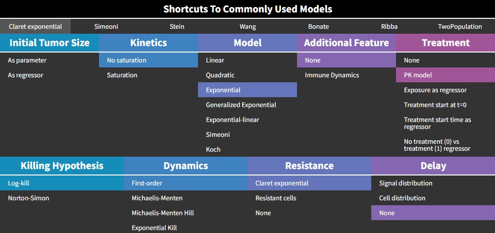
The treatment “PK model” is selected by default, but the Claret model is actually compatible with any type of treatment effect. The version with a constant treatment effect starting at t=0 (choice “Treatment start at t=0”), has an analytical solution implemented in the mode, and is therefore much faster to compute than other models implemented as ODEs
}")
-
Simeoni model
This model from Simeoni et al., 2004 corresponds to the following choices in the library:
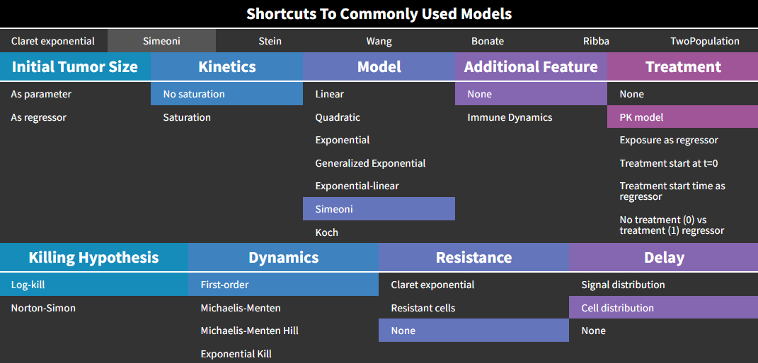
Here again, the treatment “PK model” is selected by default, but the Simeoni model is actually compatible with any type of treatment effect.
The equations are:
=TS0 \\ TS_1(t_0)=0 \\ TS_2(t=0)=0 \\ TS_3(t=0)=0 \\ \frac{dTS}{dt} = \frac{kge*TS}{(1+(\frac{kge}{kgl}*TS)^\psi)^\frac{1}{\psi}} - K*TS \\ \frac{dTS_1}{dt} = \frac{kge*TS}{(1+(\frac{kge}{kgl}*TS)^\psi)^\frac{1}{\psi}} - \frac{TS_1}{\tau} \\ \frac{dTS_2}{dt} = \frac{TS_1 - TS_2}{\tau} \\ \frac{dTS_3}{dt} = \frac{TS_2 - TS_3}{\tau} \\ TotalTS = TS+TS_1+TS_2+TS_3")
-
Two-population model
Also called evolutionary model, this simple model corresponds to an exponential growth, and a treatment effect based on log-cell kill hypothesis with first-order kinetics and no delay. The treatment can be set by the user as constant or exposure-dependent.
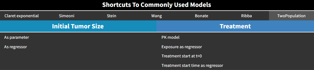
The equations are:
 \\ TSr_0 = TS0*f \\ \frac{dTS}{dt} = -kkill*EXPOSURE*TS \\ \frac{dTSr}{dt} = kge*TSr \\ TotalTS = TS+TSr")
TS represents the sensitive part of the tumor, and TSr the resistant part. TotalTS is the total tumor size.
If the treatment is constant and starts at time 0, the model is encoded with its analytical solution:
 + (1-f)*exp(-kkill*t))")
with kkill=0 before t=0.
-
Stein regression-growth model
This model from Stein et al., 2011 is a simple phenomenological equation based on the assumption that the change of tumor size during therapy results from two independent component processes: an exponential decrease/regression and an exponential regrowth of the tumor:
 + exp(kge*t) -1)")
with kkill=0 before t=0.
This model is only available with the treatment option “Treatment start at t=0”.
In responding tumors, regression dominates from start of therapy until nadir, growth dominating after nadir. Theoretical curves depicting the separate components of the model and how these combine together to give the time dependence of the tumor size appear in the figure below.
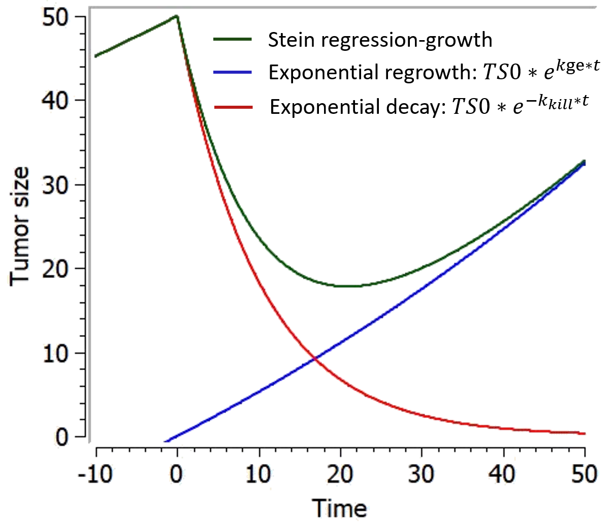
-
Wang model
This model from Wang et al., 2009 combines an exponential-decay (shrinkage) and a linear-growth (progression). In the original model, the linear growth component is considered as an approximation of tumor growth under a specific treatment, with a treatment-dependent slope. In the present library, the model is implemented with the same linear growth rate before and during treatment. It goes as follows:
+kgl*t")
This model can only be used with the option “Treatment starting at time 0”.
The following figure shows a typical prediction:
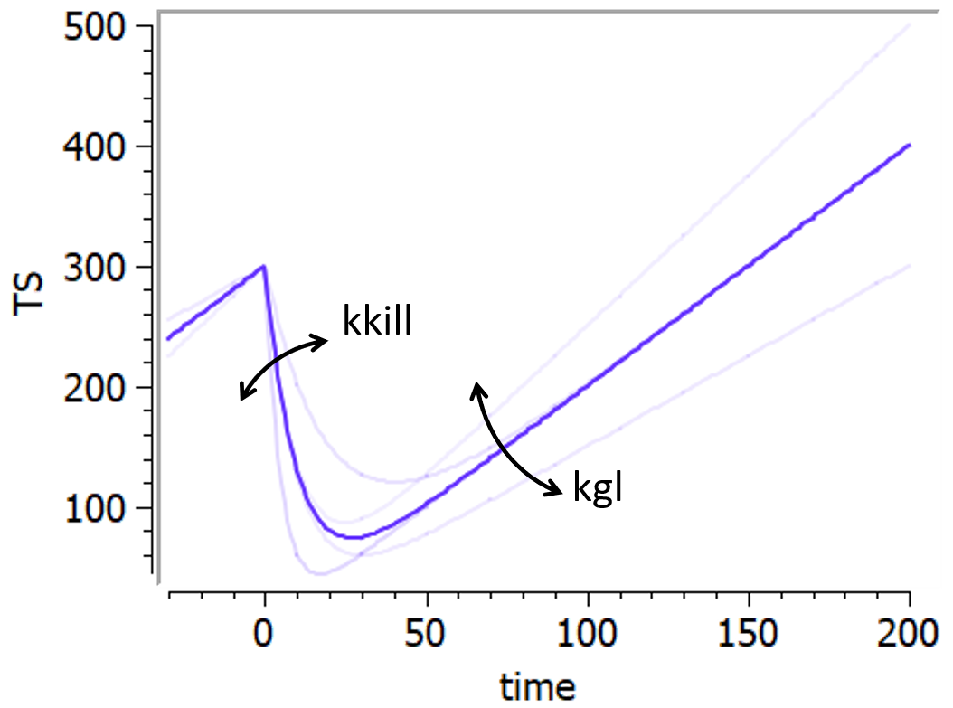
-
Bonate model
This model is based on Bonate & Suttle, 2013. It is a modification of the Wang model in which a quadratic growth term has been added to account for curvature of tumor growth following nadir.
It goes as follows:
+kgl*t+kg2*t^2")
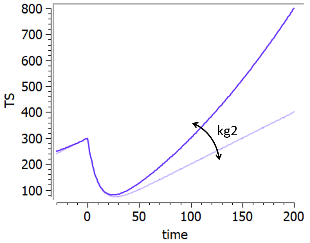
-
Ribba model
This model has been proposed by Ribba et al., 2012. It is able to capture the growth kinetics of low-grade glioma after termination of chemotherapy, characterized by a frequent decrease in volume despite chemotherapy no longer being administered, by considering delayed action of chemotherapy on quiescent tumor cells. The tumor is represented as proliferative and quiescent tumor tissues that respond differently to treatment. The treatment concentration affects both proliferative and quiescent tissue. The tissue composed of cells in proliferation is directly eliminated because of lethal DNA damages induced by the treatment. Nonproliferative tissue is also subject to DNA damages due to the treatment. When re-entering the cell cycle, the DNA-damaged quiescent cells can either repair their DNA damages and return to a proliferative state or die because of unrepaired damages.
It is represented on this figure adapted from [Ribba et al., 2012]:
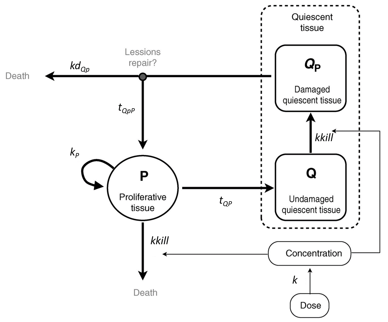
The following curves show the prediction of each variable of the model before and after a treatment dose at time 0, on the left, and the impact of the parameters on the prediction for TotalTS on the right. The treatment concentration causes an initial sharp drop in P and thus in TotalTS, as well as the transfer of cells from Q to Qp. While the treatment concentration decreases then fastly to 0, TotalTS continues decreasing slowly, driven by the elimination of Qp. TotalTS increases again only once enough cells have been transferred from Qp to P. The growth function chosen in this model includes a saturation with a carrying capacity TSmax.
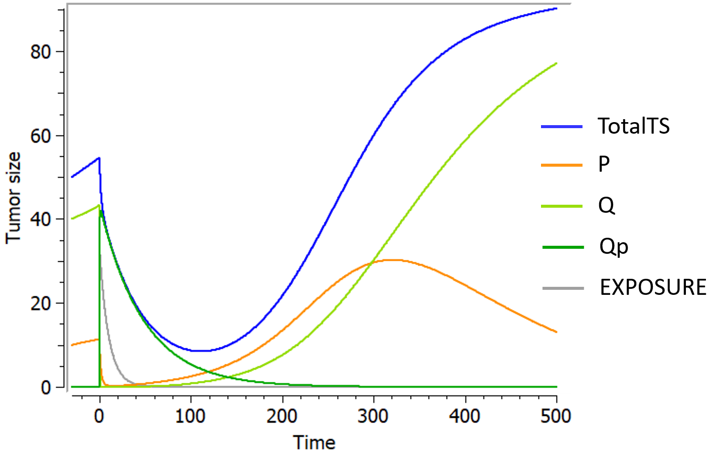
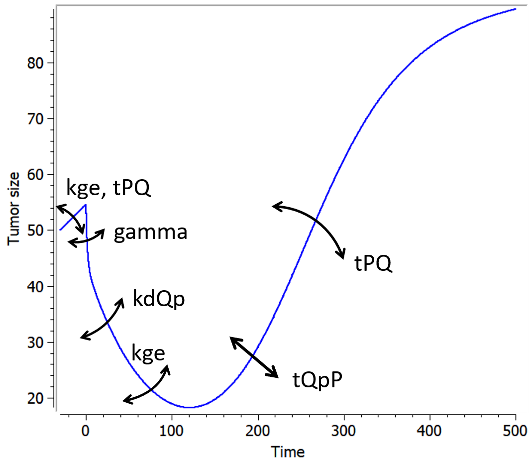
References
Reviews
- Bernard, A., Kimko, H., Mital, D., & Poggesi, I. (2012). Mathematical modeling of tumor growth and tumor growth inhibition in oncology drug development. Expert Opinion on Drug Metabolism and Toxicology, 8(9), 1057–1069.
- Ribba, B., Holford, N. H., Magni, P., Trocóniz, I., Gueorguieva, I., Girard, P., Sarr, C., Elishmereni, M., Kloft, C., & Friberg, L. E. (2014). A Review of Mixed-Effects Models of Tumor Growth and Effects of Anticancer Drug Treatment Used in Population Analysis. CPT Pharmacometrics Syst. Pharmacol.
- Benzekry, S., Lamont, C., Beheshti, A., Tracz, A., Ebos, J. M. L., Hlatky, L., & Hahnfeldt, P. (2014). Classical Mathematical Models for Description and Prediction of Experimental Tumor Growth. PLoS Computational Biology.
- Yin, A., Moes, D. J. A. R., Hasselt, J. G. C., Swen, J. J., & Guchelaar, H. (2019). A Review of Mathematical Models for Tumor Dynamics and Treatment Resistance Evolution of Solid Tumors. CPT: Pharmacometrics & Systems Pharmacology, 720–737.
- Al-Huniti, N., Feng, Y., Yu, J., Lu, Z., Nagase, M., Zhou, D., & Sheng, J. (2020). Tumor Growth Dynamic Modeling in Oncology Drug Development and Regulatory Approval: Past, Present, and Future Opportunities. CPT: Pharmacometrics and Systems Pharmacology, 1–9.
Models from literature
- Simeoni, M., Magni, P., Cammia, C., De Nicolao, G., Croci, V., Pesenti, E., Germani, M., Poggesi, I., & Rocchetti, M. (2004). Predictive pharmacokinetic-pharmacodynamic modeling of tumor growth kinetics in xenograft models after administration of anticancer agents. Cancer Research, 64(3), 1094–1101.
- Koch, G., Walz, A., Lahu, G., & Schropp, J. (2009). Modeling of tumor growth and anticancer effects of combination therapy. Journal of Pharmacokinetics and Pharmacodynamics, 36(2), 179–197.
- Haddish-Berhane, N., Shah, D. K., Ma, D., Leal, M., Gerber, H. P., Sapra, P., Barton, H. A., & Betts, A. M. (2013). On translation of antibody drug conjugates efficacy from mouse experimental tumors to the clinic: A PK/PD approach. Journal of Pharmacokinetics and Pharmacodynamics, 40(5), 557–571.
- Wheldon, T.E., 1988, Mathematical Models in Cancer Research, Adam Hilger, Bristol.
- von Bertalanffy, L. (1957). Quantitative Laws in Metabolism and Growth. The Quarterly Review of Biology, 32(3), 221–233.
- Claret L, Girard P, Hoff PM, Van Cutsem E, Zuideveld KP, Jorga K, Fagerberg J, Bruno R. Model-based prediction of phase III overall survival in colorectal cancer on the basis of phase II tumor dynamics. J Clin Oncol. 2009 Sep 1;27(25):4103-8.
- Hahnfeldt, P., Panigrahy, D., Folkman, J., & Hlatky, L. (1999). Tumor development under angiogenic signaling: A dynamical theory of tumor growth, treatment response, and postvascular dormancy. Cancer Research, 59(19), 4770–4775.
- Hahnfeldt, P., Folkman, J., & Hlatky, L. (2003). Minimizing long-term tumor burden: The logic for metronomic chemotherapeutic dosing and its antiangiogenic basis. Journal of Theoretical Biology, 220(4), 545–554.
- de Pillis, L. G., Gu, W., Fister, K. R., Head, T., Maples, K., Murugan, A., Neal, T., & Yoshida, K. (2007). Chemotherapy for tumors: An analysis of the dynamics and a study of quadratic and linear optimal controls. Mathematical Biosciences, 209(1), 292–315.
- Desmée, S., Mentré, F., Veyrat-Follet, C., & Guedj, J. (2015). Nonlinear Mixed-effect Models for Prostate-specific Antigen Kinetics and Link with Survival in the Context of Metastatic Prostate Cancer: A Comparison by Simulation of Two-stage and Joint Approaches. The AAPS Journal, 17(3), 691–699.
- Lobo, E. D., & Balthasar, J. P. (2002). Pharmacodynamic modeling of chemotherapeutic effects: Application of a transit compartment model to characterize methotrexate effects in vitro. AAPS PharmSci, 4(4), 212–222.
- Jusko, W. J. (1973). A pharmacodynamic model for cell-cycle-specific chemotherapeutic agents. Journal of Pharmacokinetics and Biopharmaceutics, 1(3), 175–200.
- Sun, Y. N., & Jusko, W. J. (1998). Transit compartments versus gamma distribution function to model signal transduction processes in pharmacodynamics. Journal of Pharmaceutical Sciences, 87(6), 732–737.
- Stein, W. D., Gulley, J. L., Schlom, J., Madan, R. A., Dahut, W., Figg, W. D., Ning, Y. M., Arlen, P. M., Price, D., Bates, S. E., & Fojo, T. (2011). Tumor regression and growth rates determined in five intramural NCI prostate cancer trials: The growth rate constant as an indicator of therapeutic efficacy. Clinical Cancer Research, 17(4), 907–917.
- Wang Y, Sung C, Dartois C, Ramchandani R, Booth BP, Rock E, Gobburu J. Elucidation of relationship between tumor size and survival in non-small-cell lung cancer patients can aid early decision making in clinical drug development. Clin Pharmacol Ther. 2009 Aug;86(2):167-74.
- Bonate, P. L., & Suttle, A. B. (2013). Modeling tumor growth kinetics after treatment with pazopanib or placebo in patients with renal cell carcinoma. Cancer Chemotherapy and Pharmacology, 72(1), 231–240.
- Ribba, B., Kaloshi, G., Peyre, M., Ricard, D., Calvez, V., Tod, M., Čajavec-Bernard, B., Idbaih, A., Psimaras, D., Dainese, L., Pallud, J., Cartalat-Carel, S., Delattre, J. Y., Honnorat, J., Grenier, E., & Ducray, F. (2012). A tumor growth inhibition model for low-grade glioma treated with chemotherapy or radiotherapy. Clinical Cancer Research, 18(18), 5071–5080.
Examples of model extensions
The TGI library implemented in Monolix has no ambition of being exhaustive. If a different or more complex TGI model is needed to capture some tumor size data, it can be convenient to start from a model defined in the library, and edit it to derive a user-custom model, a process that is straight-forward with Monolix. In this section we present a few examples of more complex models from the literature and how they can be built based on a model from the library.
Model for combination therapy
[Soon to come]
8.6.1.Additional features for tumor growth models
Dynamic carrying capacity due to angiogenesis
The library includes, as an example, a module taken from Hahnfeldt et al,1999 that models the effect of angiogenesis as a dynamic carrying-capacity. When selecting the dynamic carrying-capacity module, TSmax is defined as an ODE variable instead of a constant parameter, with the second ODE displayed on the figure below.
The first term (


On the figure, a logistic growth is used for TS, but this module can be combined with any other tumor growth model that includes the TSmax parameter (saturation).
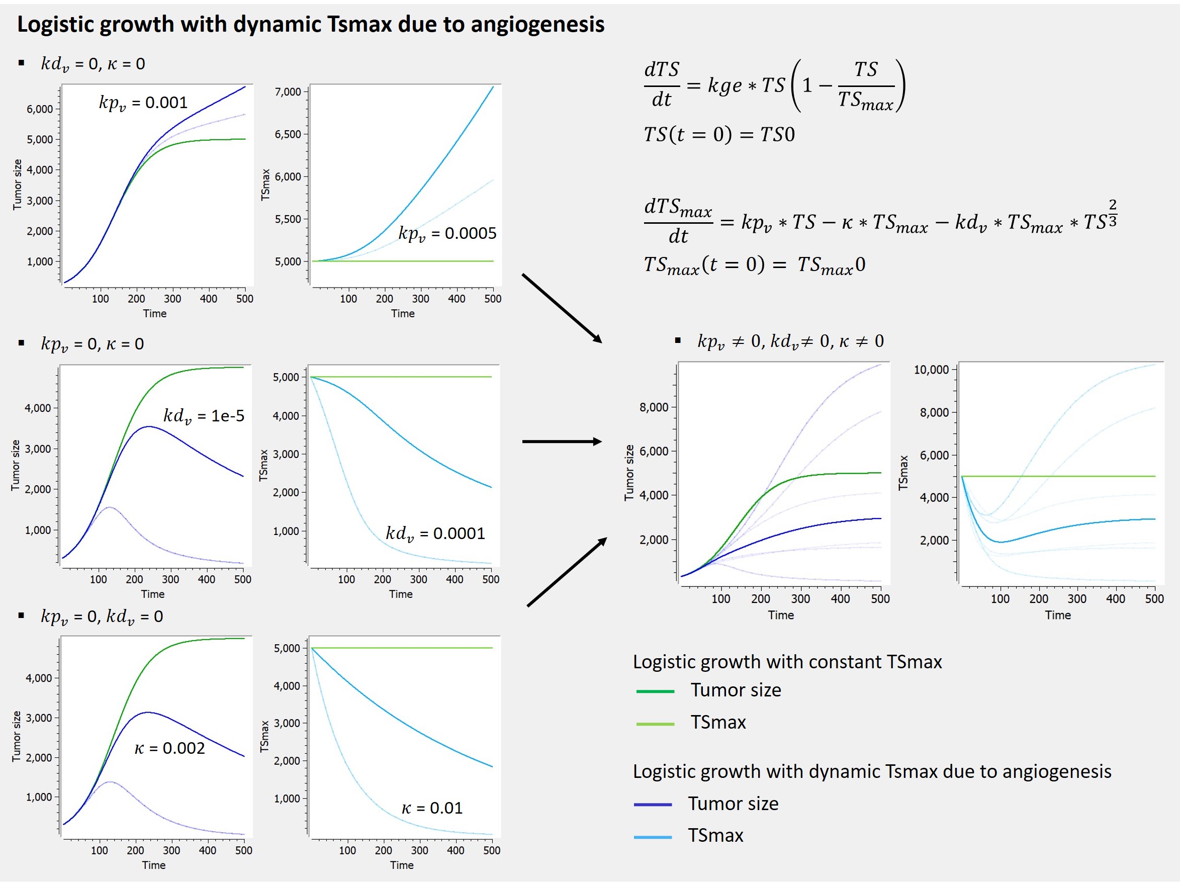
Immune dynamics causing shrinkage or oscillations of tumor size
Effector immune cell dynamics and their effect on the tumor cell population size may also be modelled as to allow for the production of certain clinically observed trends such as tumor dormancy, oscillation in tumor size and even spontaneous tumor regression.
The library includes, as an example, a model of tumor-immune interactions with chemotherapy proposed by De Pillis et al. (2007), taking into account the control of the tumor growth by the immune system, and the weakening of the immune system as a side effect of chemotherapy.
In this model, tumor cells are killed by the effector cells through a mass-action dynamic with kill rate c. The effector cells have a constant source rate kpi, while death is proportional to the population of effector cells through the term -kdi*I. Effector cells are also recruited by tumor cells through a Michaelis–Menten term, which serves to provide a saturation effect. Additionally, effector cells are inactivated through contact with tumor cells according to a mass-action dynamic with parameter p.
The corresponding ODEs are displayed on the figure below, together with predictions obtained with typical parameter values, showing the impact of the different terms in the equation governing the immune effector cells dynamics and the variety of behaviors that it can cause for the tumor cells, and the immune cells.
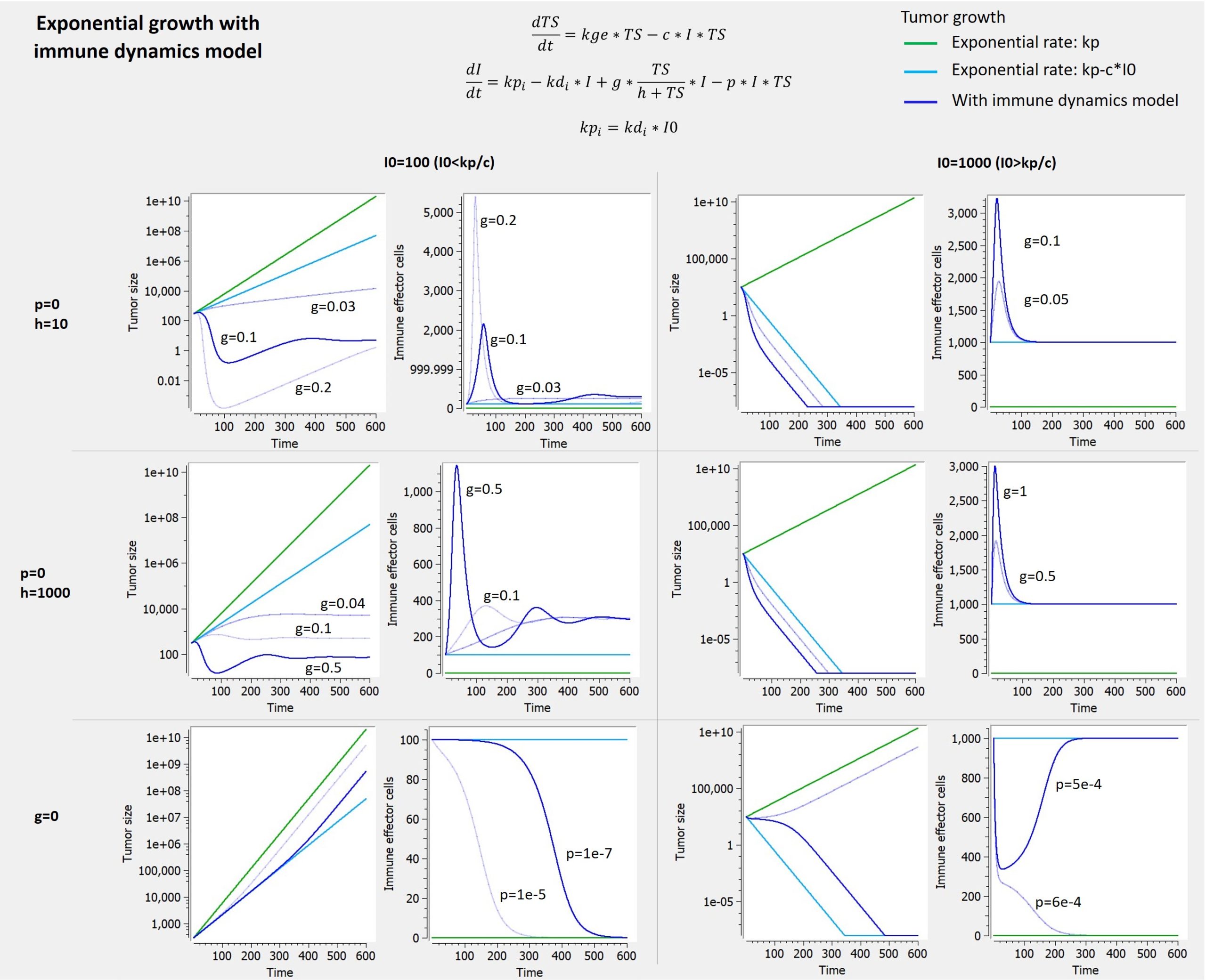
8.7.Time-to-event modeling with the MonolixSuite
This page presents the TTE model library proposed by Lixoft. It includes an introduction on time-to-event data, the different ways to model this kind of data, and typical parametric models.
|
|
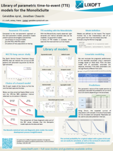
What is time-to-event data
In case of time-to-event data the recorded observations are the times at which events occur. We can for instance record the time (duration) from diagnosis of a disease until death, or the time between administration of a drug and the next epileptic seizures. In the first case, the event is one-off, while in the second it can be repeated.
In addition, the event can be:
- exactly observed: we know the event has happen exactly at time \(t_i (T_i=t_i)\)
- interval censored: we know the event has happen during a time interval, but not exactly when \((a_i \leq T_i \leq b_i)\)
- right censored: the observation period ends before the event can be observed \((T_i > t_{end}) \)
Formatting of time-to-event data in the MonolixSuite
In the data set, exactly observed events, interval censored events and right censoring are recorded for each individual. Contrary to other softwares for survival analysis, the MonolixSuite requires to specify the time at which the observation period starts. This allow to define the data set using absolute times, in addition to durations (if the start time is zero, the records represent durations between the start time and the event). 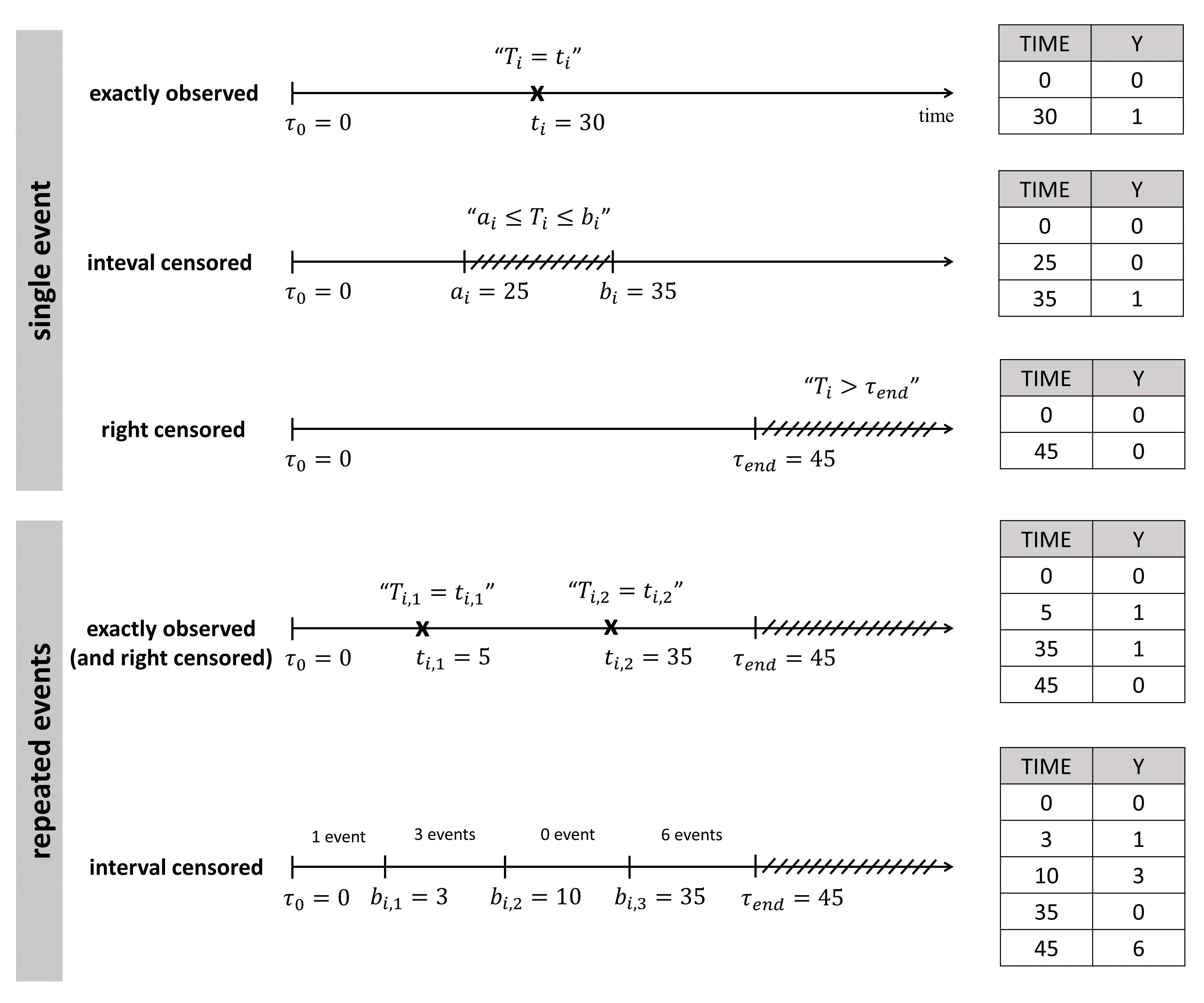
For instance for single events, exactly observed (with or without right censoring), one must indicate the start time of the observation period (Y=0), and the time of event (Y=1) or the time of the end of the observation period if no event has occurred (Y=0). In the following example:
ID TIME Y
1   0   0
1  34   1
2   0   0
2  80   0
the observation period last from starting time t=0 to the final time t=80. For individual 1, the event is observed at t=34, and for individual 2, no event is observed during the period. Thus it is indicated that at the final time (t=80), no event had occurred. Using absolute times instead of durations, we could equivalently write:
ID TIME Y
1  20   0
1  54   1
2  33   0
2  113  0
The durations between start time and event (or end of the observation period) are the same as before, but this time we record the day at which the patients enter the study and the days at which they have events or leave the study. Different patients may enter the study at different times.
Important concepts: hazard and survival
Two functions have a key role in time-to-event analysis: the survival function and the hazard function. The survival function S(t) is the probability that the event happens after time t. A common way to estimate it non-parametrically is to calculate the Kaplan-Meier estimate. The hazard function h(t) is the instantaneous rate of an event, given that it has not already occurred. Both are linked by the following equation:
$$S(t)=e^{-\int_0^t h(x) dx}$$
Different types of approaches
Depending on the goal of the time-to-event analysis, different modeling approaches can be used: non-parametric, semi-parametric (Cox models) and parametric.
- Non-parametric models do not require assumptions on the shape of the hazard or survival. Using the Kaplan-Meier estimate, statistical tests can be performed to check if the survival differs between sub-populations. The main limitations of this approach are that (i) only categorical covariates can be tested and (ii) the way the survival is affected by the covariate cannot be assessed.
- Semi-parametric models (Cox models) assume that the hazard can be written as a baseline hazard (that depends only on time), multiplied by a term that depends only on the covariates (and not time). Under this hypothesis of proportional covariate effect, one can analyze the effect of covariates (categorical and continuous) in a parametric way, leaving the baseline hazard undefined.
- Parametric models require to fully specify the hazard function. If a good model can be found, statistical tests are more powerful than for semi-parametric models. In addition, there is no restrictions on how the covariates affects the hazard. Parametric models can also be easily used for predictions.
The table below synthesizes the possibilities for the 3 approaches.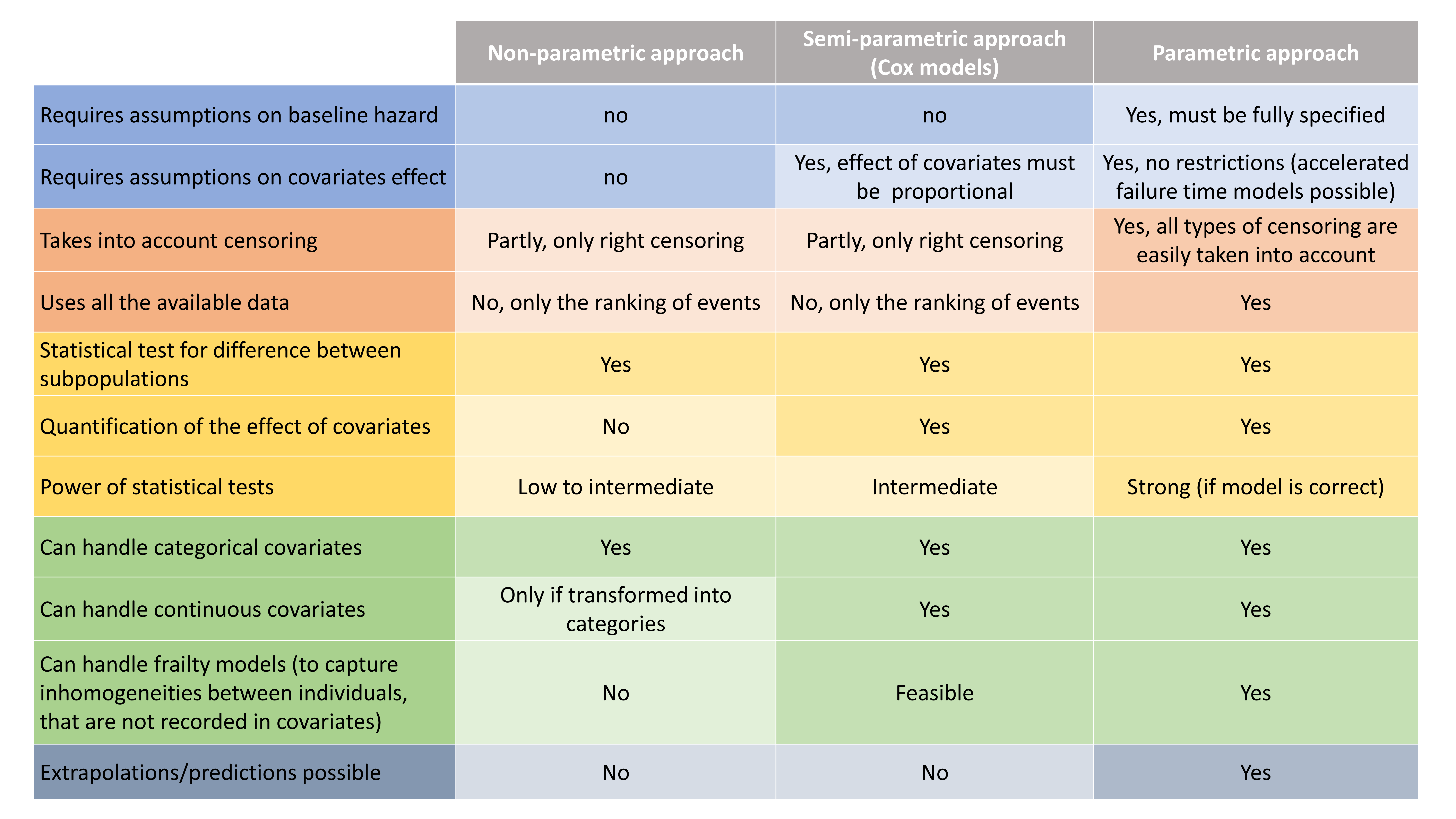
Focus on parametric modeling with the MonolixSuite
In the MonolixSuite, the only possible approach is the parametric approach. The model is defined via the hazard function, which in a population approach typically depends on individual parameters: \(h(t,\psi_i)\). With the hazard function, the survival function can easily be computed, as well as the conditional distribution \(p_{y_i|\psi_i}\) for various censoring situations (which is required for parameter estimation via SAEM, log-likelihood calculation, etc).
The typical syntax to define the output is the following:
DEFINITION:
Event = {type=event, maxEventNumber=1, hazard=h}
The output Event will be matched to the time-to-event data of the data set. The hazard function h is usually defined via an expression including the input individual parameters. For one-off events, the maximal number of events per individual is 1. It is important to indicate it in the maxEventNumber argument to speed up calculations. To use the model for simulations with Simulx, rightCensoringTime must be given as additional argument. Check here for details.
Note that the hazard can be a function of other variables such as drug concentration or tumor burden for instance (joint PK-TTE or PD-TTE models). An example of the syntax is given here.
Library of parametric models for time-to-event data
To describe the various shapes that the survival Kaplan-Meier estimate can take, several hazard functions have been proposed. Below we display the survival curves, for the most typical hazard functions:
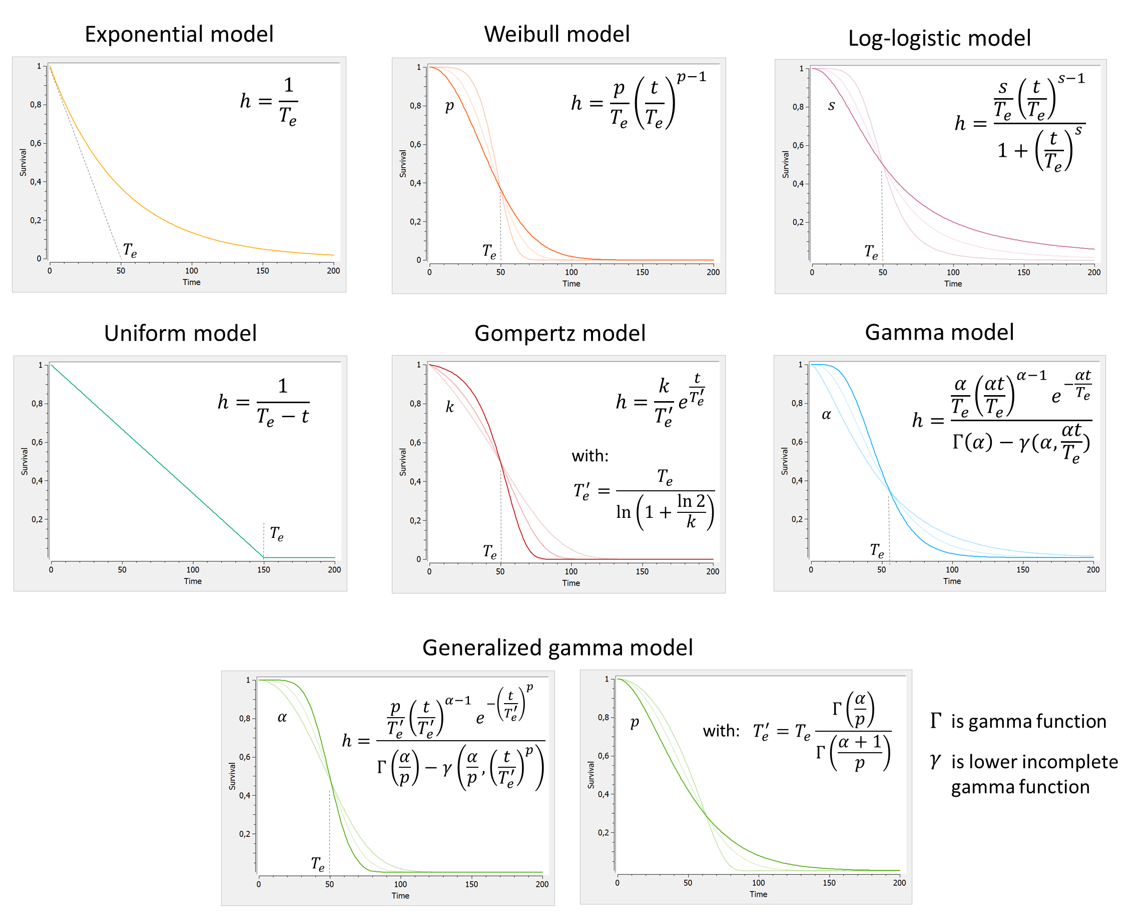
A few comments:
- We have reparametrized \(T_e’\) as a function of \(T_e\) to better separate the effects of the scale parameter (characteristic time) and the shape parameter (shape of the curve).
- All parameters are positive. If we assume inter-individual variability, a log-normal distribution is usually appropriate.
The table below summarizes the number of parameters and typical parameter values: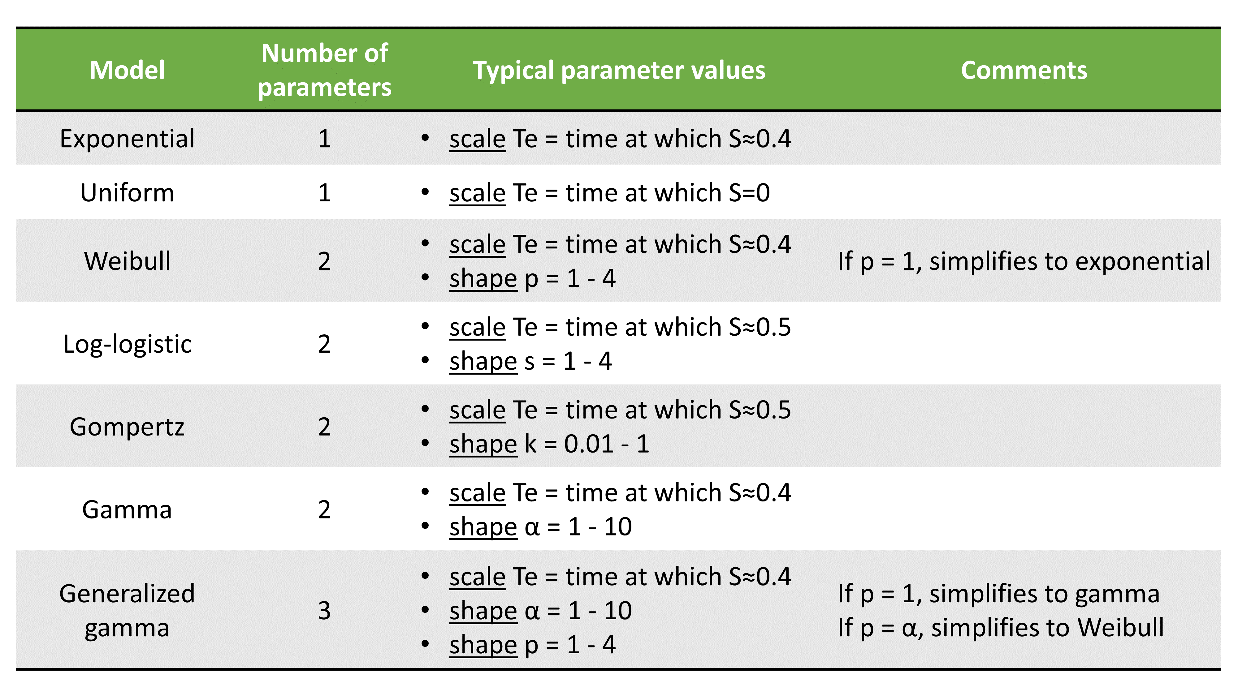
For each model, we can in addition consider a delay del as additional parameter. The delay will simply shift the survival curve to the right (later times). For t<del, the survival is S(t<del)=1.
Downloads:
These models can be explore in Mlxplore (download Mlxplore project here). A shiny-mlxR app also permits to give any hazard function and visualize the corresponding survival curve (click here).
All models are available as Mlxtran model file in the TTE library. Each model can be with/without delay and for single/repeated events. For performance reasons, it is important to choose the file ending with ‘_singleEvent.txt’ if you want to model one-off events (death, drop-out, etc).
Case studies
Two case studies show the modeling and simulation workflow for TTE data:
8.8.Count data modeling with the MonolixSuite
This page presents the count model library proposed by Lixoft from the 2019 version on. It includes a short introduction on count data, the different ways to model this kind of data, and typical models.
- What is count data
- Formatting of count data in the MonolixSuite
- Important concepts: the probability mass function
- Encoding of count models in the MonolixSuite
- Library of parametric models for count data
- Case studies
What is count data
Count data come from counting something, e.g., the number of trials required for completing a given task. The task can for instance be repeated several times (longitudinal count data) and the individuals performance followed.
Count data can also represent the number of events happening in regularly spaced intervals, e.g the number of seizures every week. If the time intervals are not regular, the data may be considered as repeated time-to-event interval censored, or the interval length can be given as regressor to be used to define the probability distribution in the model.
Formatting of count data in the MonolixSuite
Count data can take only non-negative integer values. The counts for each individual are recorded in the OBSERVATION column-type. If the data is longitudinal (over time), the times at which the counts have been recorded are indicated in the TIME column-type. If the data is not longitudinal, the TIME column is still necessary and a time of 0 can be used for instance.
ID TIME Y
1   0   8
1   4   9
1   8   11
2   0   6
2   4   6
2   8   7
In the example above, the values in the time column can either indicate the time at which the counts have been counted, or the start or end time of the period over which the number of events are recorded.
In the Monolix GUI, the user must indicate that the data is of type Count/Categorical:
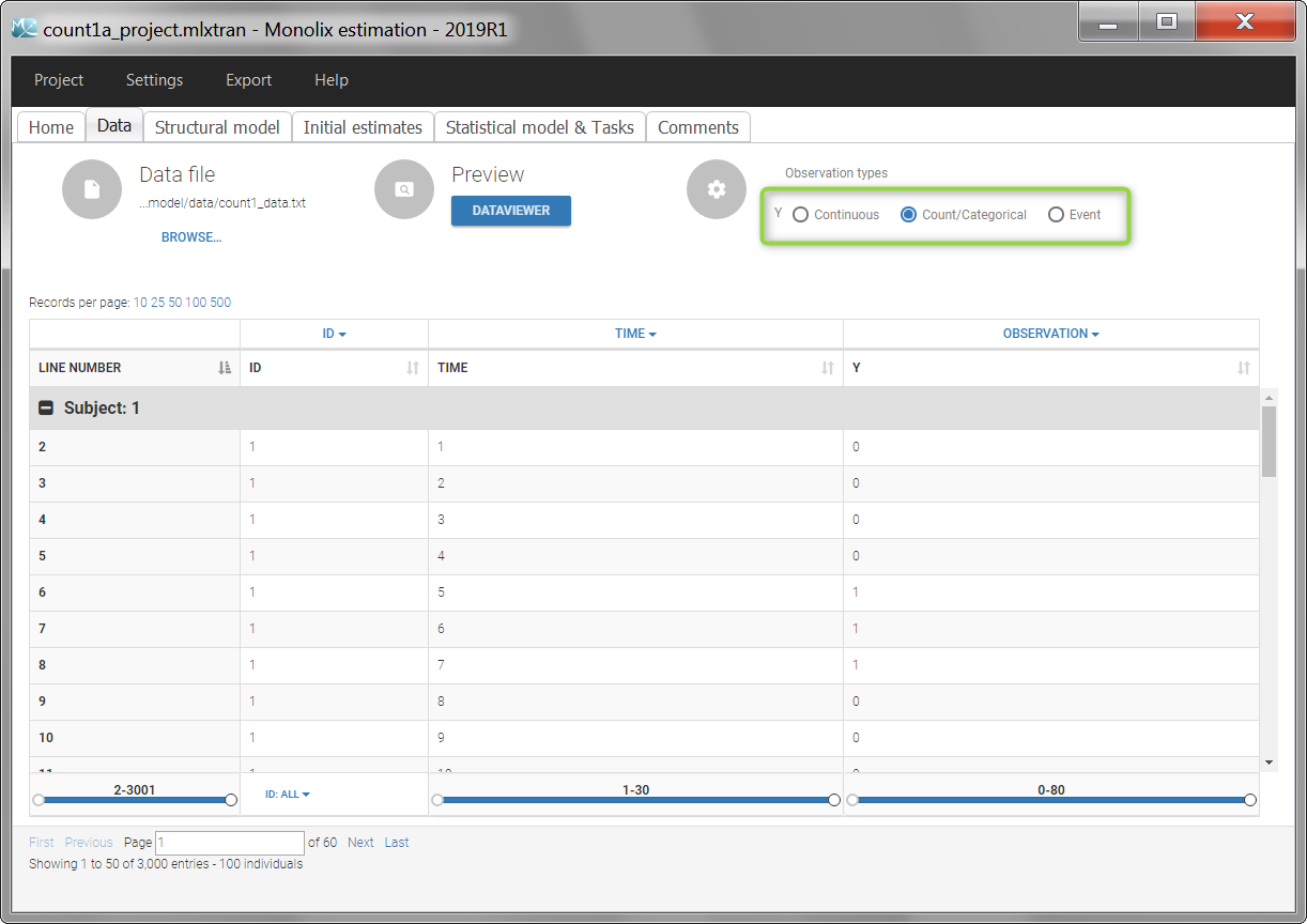
Important concept: the probability mass function
Count data are described by their probability mass function, which gives the probability that the discrete random variable is exactly equal to some value: \( \mathbb{P}(y_{ij}=k) \) with \(y_{ij}\) the observed count number for individual \(i\) at time \(j\) and \(k>0\).
For instance the probability mass function for a Poisson distribution is:
\(\mathbb{P}(y_{ij}=k)=\frac{\lambda^k e^{-\lambda}}{k!} \)
If \(\lambda=3\), then the probability of having a count of 0 is 4.9%, a count of 1 is 14.9%, a count of 2 is 22.4%, a count of 3 is 22.4%, etc.
Encoding of count models with the MonolixSuite
In Monolix, a model for count data is defined via the probability mass function, which in a population approach typically depends on individual parameters: \( \mathbb{P}(y_{ij}=k) = f(t_j,\psi_i)\).
The typical syntax to define the random variable representing the count number is the following:
DEFINITION:
CountNumber = {type=count, P(CountNumber=k) = ...}
CountNumber is the name of the random variable and can be replaced by another name. On the opposite, k is a mandatory name for the values. The random variable CountNumber is then listed in the outputs, to be matched to the observed data.
The probability mass functions often involve ratios of factorials. While the ratio is often a reasonable value, the numerator and denominator can be huge values that are difficult to handle numerically. It is therefore better to work with the log of the factorials. The function for log factorial in Mlxtran language is factln() (for integers). To extend the factorials to the continuous domain, the gamma function can be useful: \( \Gamma(n)=(n-1)!\). The log of the gamma function corresponds to the gammaln() function in Mlxtran. It is possible to define directly the log of the probability mass function with:
DEFINITION:
CountNumber = {type=count, log(P(CountNumber=k)) = ...}
For instance to define a binomial distribution, we can write:
DEFINITION:
Y = {type=count, log(P(Y=k)) = gammaln(n+1) - factln(k) - gammaln(n-k+1) + k*log(p) + (n-k)*log(1-p)}
where gammaln() is used for terms that can be non-integers and factln() for terms that are integers.
It is possible to use “if” statements related to \(k\) in the definition of the probability mass function by using the syntax below. This can be useful to define zero-inflated models for instance. The “if” statements relating to time, regressors, or parameters values can be put in a EQUATION: section before the DEFINITION: block.
DEFINITION:
CountNumber = {type=count,
if k==0
Pk = ...
else
Pk = ...
end
P(CountNumber=k) = Pk}
The parameters involved in the definition of the probability mass function (for instance \(\lambda\) for a Poisson distribution) can be identical for all individuals, or vary from individual to individual. This is defined in the section “Individual model” of the graphical interface as usual. These parameters can also evolve over time or be a function of other variables such as drug concentration or tumor burden for instance. See the demo “PKcount_project.mlxtran” for instance in the Monolix demo folder, section 4.2.
Library of models for count data
To describe the various shapes that a count distribution can take, we have developed a library of models. The library includes the most typical distributions, their zero-inflated counterpart, and several options for the evolution of time of the main parameter:
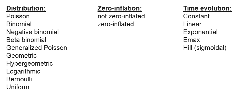
The probability mass functions and a description of the parameters is given below:

Case studies
[coming soon]
9.Examples
Different examples of full models are presented here to show how to use the Mlxtran language to define a model. When relevant, an Mlxplore project is also given, for model exploration.
Models from library
Classical extensions
Advanced models
- lifespan models
- K-PD models
- parent-metabolite model
- tumor growth model
- Friberg model for myelosupression
- ADC model
Other examples
9.1.PK models with peripheral compartments
Given a central compartment defined using the compartment macro, peripheral compartments can be defined using the peripheral macro. To define rates between peripheral compartments, the transfer macro can be used.
Model with 2 peripheral compartments connected to the central compartment

This model is available in the library and can be defined using the pkmodel macro. The model can also be defined using a set of macros:
[LONGITUDINAL]
input = {V, k12, k21, k13, k31, k}

PK:
compartment(cmt=1, volume=V, concentration=Cc)
peripheral(k12, k21)
peripheral(k13, k31)
elimination(cmt=1, k)
iv(cmt=1)

OUTPUT:
output=Cc
Note that peripheral(k12, k21) implicitly defines compartment number 2 (no need to write compartment(cmt=2)). The integers i and j used in the parameter name kij (e.g 1 and 2 for k12) indicate that compartment i is connected to compartment j.
To use macro constant instead, the macro constant can be passed as input parameters, transformed into micro constant that are themselves used in the macros.
[LONGITUDINAL]
input = {V1, Cl, Q2, V2, Q3, V3}

PK:
compartment(cmt=1, volume=V1, concentration=Cc)
peripheral(k12=Q2/V1, k21=Q2/V2)
peripheral(k13=Q3/V1, k31=Q3/V3)
elimination(cmt=1, Cl)
iv(cmt=1)

OUTPUT:
output=Cc
Model for 2 peripheral compartments in a row
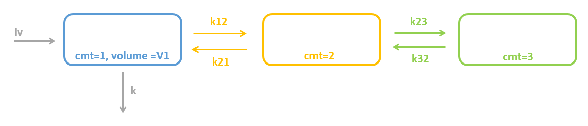
To model two peripheral compartments in a row, two peripheral macros can be used: peripheral(k12, k21) creates compartment number 2 and connects it to compartment number 1; and peripheral(k23, k32) creates compartment number 3 and connects it to compartment number 2.
[LONGITUDINAL]
input = {V, k12, k21, k23, k32, k}

PK:
compartment(cmt=1, volume=V, concentration=Cc)
peripheral(k12, k21)
peripheral(k23, k32)
elimination(cmt=1, k)
iv(cmt=1)

OUTPUT:
output=Cc
The model can also be parameterized with macro constants:
[LONGITUDINAL]
input = {V1, Cl, Q2, V2, Q3, V3}

PK:
compartment(cmt=1, volume=V1, concentration=Cc)
peripheral(k12=Q2/V1, k21=Q2/V2)
peripheral(k23=Q3/V2, k32=Q3/V3)
elimination(cmt=1, Cl)
iv(cmt=1)

OUTPUT:
output=Cc
Model with 2 interconnected peripheral compartments
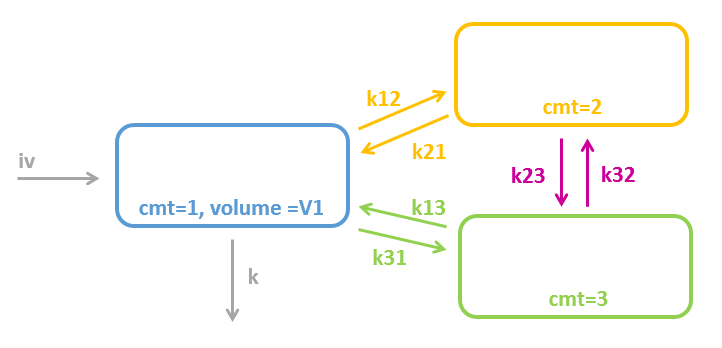
To define a model with 2 interconnected peripheral compartments, it is not possible to use only peripheral macros. Indeed, when writing:
;=== does not work ===
peripheral(k12, k21)
peripheral(k13, k31)
peripheral(k23, k32)
the third line peripheral(k23, k32) would try to create a compartment number 3, which already exists (defined by peripheral(k13, k31)). This would result into an error “conflicting compartment definition”.
Instead we can use the transfer macro:
[LONGITUDINAL]
input = {V, k12, k21, k13, k31, k23, k32, k}

PK:
compartment(cmt=1, volume=V, concentration=Cc)
peripheral(k12, k21)
peripheral(k13, k31)
transfer(from=2, to=3, kt=k23)
transfer(from=3, to=2, kt=k32)
elimination(cmt=1, k)
iv(cmt=1)

OUTPUT:
output=Cc
Model with eliminations from the central and peripheral compartments

To model a double elimination from the central and the peripheral compartments, the macro elimination can just be written twice, with the argument cmt=1 and cmt=2.
[LONGITUDINAL]
input = {V, k12, k21, k1, k2}

PK:
compartment(cmt=1, volume=V, concentration=Cc)
peripheral(k12, k21)
elimination(cmt=1, k1)
elimination(cmt=2, k2)
iv(cmt=1)

OUTPUT:
output=Cc
9.2.PK/PD model with indirect response
When the response to a drug is not directly related to the drug’s concentration (or to the concentration in a effect compartment), indirect response models have been proposed. The response R is assumed to be produced by a zero-order synthesis rate and degraded via a first-order process:

The baseline response is 
The drug can act on kin or kout by inhibition or stimulation, leading to 4 situations:
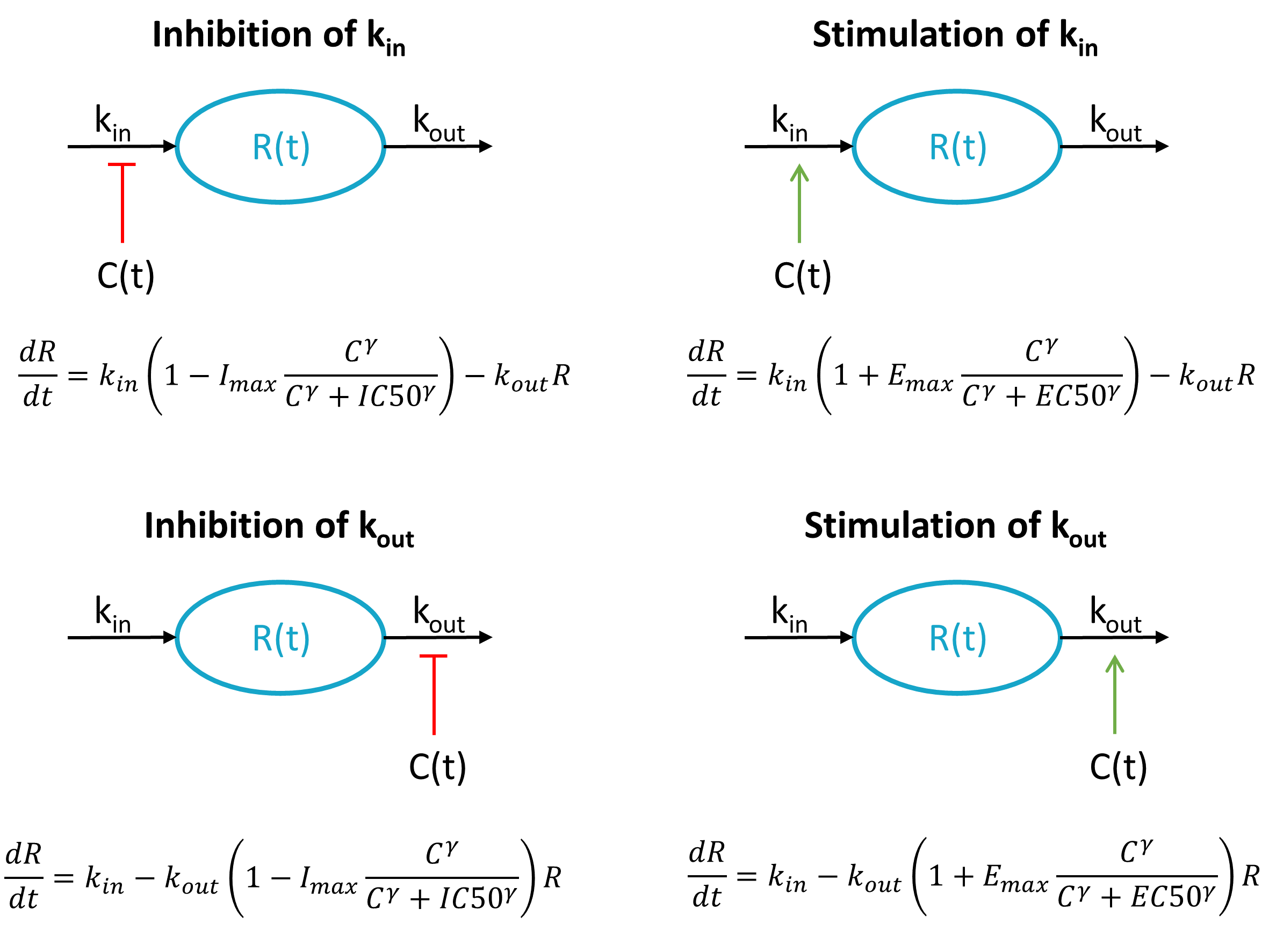
Each of these 4 cases have been presented and analysed in Dayneka et al. (1993).
Mlxtran models
Below we present the mlxtran code for each situation, in the case of a bolus administration of the drug and one compartment. The PK part of the model can easily be modified to represent more complex pharmacokinetics.
We here assume that both the drug concentration (tagged with YTYPE=1 in the data set) and the response (tagged with YTYPE=2) have been measured. If only the response is measured, the only output is R (i.e output={R}). Note that the system can also be parameterized with (R0, kin) instead of (kin,kout). Imax must be bound between 0 and 1, such that a logit distribution is most appropriate.
Inhibition of kin
[LONGITUDINAL]
input = {V, k, kin, kout, Imax, IC50, gamma}

EQUATION:
Cc = pkmodel(V,k)

odeType=stiff
t_0 = 0
R_0 = kin/kout

ddt_R = kin*(1-Imax*Cc^gamma/(Cc^gamma + IC50^gamma)) - kout*R

OUTPUT:
output = {Cc, R}
Inhibition of kout
[LONGITUDINAL]
input = {V, k, kin, kout, Imax, IC50, gamma}

EQUATION:
Cc = pkmodel(V,k)

odeType=stiff
t_0 = 0
R_0 = kin/kout

ddt_R = kin - kout*(1-Imax*Cc^gamma/(Cc^gamma + IC50^gamma))*R

OUTPUT:
output = {Cc, R}
Stimulation of kin
[LONGITUDINAL]
input = {V, k, kin, kout, Emax, EC50, gamma}

EQUATION:
Cc = pkmodel(V,k)

odeType=stiff
t_0 = 0
R_0 = kin/kout

ddt_R = kin*(1+Emax*Cc^gamma/(Cc^gamma + EC50^gamma)) - kout*R

OUTPUT:
output = {Cc, R}
Stimulation of kout
[LONGITUDINAL]
input = {V, k, kin, kout, Emax, EC50, gamma}

EQUATION:
Cc = pkmodel(V,k)

odeType=stiff
t_0 = 0
R_0 = kin/kout

ddt_R = kin - kout*(1+Emax*Cc^gamma/(Cc^gamma + EC50^gamma))*R

OUTPUT:
output = {Cc, R}
Model exploration with Mlxplore
The 4 models have been implemented in an Mlxplore project for comparison. The Mlxplore script reads:
<MODEL>
[LONGITUDINAL]
input = {V, k, kin, kout, Imax1, IC501, gamma1, Imax2, IC502, gamma2, Emax3, EC503, gamma3, Emax4, EC504, gamma4}

EQUATION:
Cc=pkmodel(V,k)

odeType=stiff
t_0 = 0
R1_0 = kin/kout
R2_0 = kin/kout
R3_0 = kin/kout
R4_0 = kin/kout

ddt_R1 = kin*(1-Imax1* Cc^gamma1/(Cc^gamma1+IC501^gamma1)) - kout*R1
ddt_R2 = kin - kout*(1-Imax2* Cc^gamma2/(Cc^gamma2+IC502^gamma2))*R2
ddt_R3 = kin*(1+Emax3* Cc^gamma3/(Cc^gamma3+EC503^gamma3)) - kout*R3
ddt_R4 = kin - kout*(1+Emax4* Cc^gamma4/(Cc^gamma4+EC504^gamma4))*R4

<PARAMETER>
V = 10
k = 0.1
kin = 10
kout = 1
Imax1 = 0.8
IC501 = 10
gamma1 = 2
Imax2 = 0.8
IC502 = 10
gamma2 = 2
Emax3 = 3
EC503 = 10
gamma3 = 2
Emax4 = 3
EC504 = 10
gamma4 = 2

<DESIGN>
[ADMINISTRATION]
adm100 = {time=0, amount=100}
adm200 = {time=0, amount=200}
adm300 = {time=0, amount=300}

<OUTPUT>
list={R1,R2,R3,R4}
grid=0:0.1:60

<RESULTS>
[GRAPHICS]
p1 = {y={R1}, ylabel='inhibition of kin', xlabel='time'}
p2 = {y={R4}, ylabel='stimulation of kout', xlabel='time'}
p3 = {y={R2}, ylabel='inhibition of kout', xlabel='time'}
p4 = {y={R3}, ylabel='stimulation of kin', xlabel='time'}
The resulting dynamics of the response for 3 different doses for each model is depicted below:
9.3.PK/PD model with effect compartment
Mlxtran structural model
The model can be defined either using the pkmodel macro or a combination of several other macros used as building blocks.
Using the pkmodel macro
[LONGITUDINAL]
input = {ka, V, k, k12, k21, ke0, Emax, EC50, gamma}

PK:
{Cc, Ce} = pkmodel(ka,V,k,k12, k21,ke0)

EQUATION:
Effect = Emax*Ce^gamma/(Ce^gamma+EC50^gamma)

OUTPUT:
output = {Cc, Effect}
The PK part of the model (including the effect compartment) can easily be defined using the pkmodel macro, which infers the model based on the input keywords. With {Cc, Ce} = pkmodel(ka,V,k,k12, k21,ke0), we define a 2-compartment model with first-order absorption and linear elimination, as well as an effect compartment. The concentrations in the central compartment and in the effect compartment are outputted by the macro and can be used to define the PD part of the model.
The PD part of the model (the effect) is defined via an analytical expression which takes into account the concentration in the effect compartment Ce.
Using macros
Instead of using the pkmodel macro, the PK part of the model can also be defined using other macros as building blocks.
[LONGITUDINAL]
input = {ka, V, k, k12, k21, ke0, Emax, EC50, gamma}

PK:
compartment(cmt=1, volume=V, concentration=Cc)
oral(cmt=1, ka)
elimination(cmt=1,k)
peripheral(k12,k21)
effect(cmt=1,ke0,concentration=Ce)

EQUATION:
Effect = Emax*Ce^gamma/(Ce^gamma+EC50^gamma)

OUTPUT:
output = {Cc, Effect}
Model exploration using Mlxplore
The Mlxplore script including the parameter values, administration design (here one dose) and output reads:
<MODEL>
[LONGITUDINAL]
input = {ka, V, k, k12, k21, ke0, Emax, EC50, gamma}

PK:
{Cc, Ce} = pkmodel(ka,V,k,k12, k21,ke0)

EQUATION:
Effect = Emax*Ce^gamma/(Ce^gamma+EC50^gamma)

OUTPUT:
output = {Cc, Effect}

<PARAMETER>
ka = 1
V = 10
k = 0.1
k12 = 0.05
k21 = 0.05
ke0 = 0.1
Emax = 15
EC50 = 1
gamma = 2

<DESIGN>
[ADMINISTRATION]
adm = {time=0, amount=100}

<OUTPUT>
list={Cc,Ce,Effect}
grid=0:0.1:60

<RESULTS>
[GRAPHICS]
p1 = {y={Cc,Ce}, ylabel='Concentrations Cc, Ce', xlabel='Time'}
p2 = {y={Effect}, ylabel='Effect', xlabel='Time'}
Below we visualize the impact of a reduction of the parameter ke0, leading to a longer delay in the appearance of the compound in the effect compartment:
One can also plot the effect with respect to the concentration in the central compartment by changing the <RESULTS> section to:
<RESULTS>
[GRAPHICS]
p1 = {y={Effect}, x={Cc}, ylabel='Effect', xlabel='Concentration Cc'}
Using the ‘animation’ button, the hysteresis characteristic of delayed responses can be visualized:
9.4.Model with mixed first-order and zero-order absorption, or parallel first-order
Some drugs can display complex absorption kinetics. Common examples are mixed first-order and zero-order absorptions, wheer one fraction of the dose is absorbed via one route and the other fraction via another route, either simultaneously or with one of the route showing a delay. Another example is fast and slow first-order absorptions in parallel. Finally, sequential absorption with a zero-order process into a transit compartment followed by a first-order absorption in the central compartment is also possible.
A few examples of those kinds of absorption kinetics are listed below:
- parallel first-order: oral sustained-release Diltiazem (Murata et al. 1989) and sublingual doses with a rapid absorption from the bucal cavity followed by a delayed absorption from the gastrointestinal tract (“Pharmacokinetic and Pharmacodynamic Data Analysis: Concepts and Applications” by Gabrielsson and Weiner)
- first-order followed by zero-order: oral sumatriptan (Cosson et al. 1999)
- zero-order followed by first-order: oral cefadroxil (Guarrigues et al. 1991)
More examples of complex absorptions are given in:
Mlxtran models
For the examples below, we consider a single compartment and a linear elimination. The model is described using macros. When two absorption routes are considered, a fraction F of the dose is absorbed via the one process and the remaining 1-F fraction of the dose is absorbed via another process. In the data set, the dose lines must not be duplicated. A single dose line can be split into two processes using the keyword p in the absorption macros.
As the parameter F must stay within [0,1], a logit distribution must be chosen in the Monolix GUI.
Sequential absoption
In this model, the drug is first absorbed via a zero-order process into a transit compartment and then transferred from the transit compartment into the central compartment using a first-order process. This model allows to capture a progressively faster increase of the concentration during the absorption phase with a simpler model than when taking into account an estimated number of transit compartments (absorption macro with Mtt and Ktr parameters). In addition, this model has the advantage of using an analytical solution, so it is faster to run than a model with estimated transit compartmet that require the solve an ODE system. For the analytical solution to be used, a dummy elimination (equal to zero) from the transit compartment is necessary.
[LONGITUDINAL]
input = {Tk0, ka, V, Cl}
PK:
compartment(cmt = 1, amount = Ad)
oral(cmt = 1, Tk0)
elimination(cmt = 1, Cl=0) ; dummy elimination term
compartment(cmt = 2, volume = V, concentration = Cc)
transfer(from = 1, to = 2, kt = ka)
elimination(cmt = 2, Cl)
OUTPUT:
output = {Cc}
This model is not yet available in the Monolix libraries.
Parallel first-order
Parallel first-order absorptions can have various causes, among other: absorption via water and lipid routes for dermal administrations, absorption in the bucal cavity and GI tract for sublingual administrations, progressive solubilisation along the GI tract and subsequent intestinal absorption for oral administrations or simply two different absorption sites.
[LONGITUDINAL]
input = {ka1, ka2, Tlag, F, V, Cl}

PK:
compartment(cmt=1, volume=V, concentration=Cc)
absorption(cmt=1, ka=ka1, p=F)
absorption(cmt=1, ka=ka2, Tlag, p=1-F)
elimination(cmt=1, Cl)

OUTPUT:
output = {Cc}
This model is available in the PK double absorption library, with the name oral1_oral1_1cpt_ka1ka2F1Tlag2VCl.txt, with Tlag named Tlag2 and F named F1.
Simultaneous zero-order and first-order
The drug is simultaneously absorbed via a first-order and a zero-order process, which both start at the administration time (no lag time).
[LONGITUDINAL]
input = {ka, Tk0, F, V, Cl}

PK:
compartment(cmt=1, volume=V, concentration=Cc)
absorption(cmt=1, Tk0, p=F)
absorption(cmt=1, ka, p=1-F)
elimination(cmt=1, Cl)

OUTPUT:
output = {Cc}
This model is available in the PK double absorption library, with the name oral0_oral1_1cpt_Tk01ka2F1VCl.txt, with Tk0 named Tk01, ka named ka2, and F named F1.
Sequential zero-order followed by first order
The drug is first absorbed via a zero-order process during a time Tk0. Once this is finished, the remaining fraction is absorbed via a first-order process, which starts with a lag time Tk0.
[LONGITUDINAL]
input = {ka, Tk0, F, V, Cl}

PK:
compartment(cmt=1, volume=V, concentration=Cc)
absorption(cmt=1, Tk0, p=F)
absorption(cmt=1, Tlag=Tk0, ka, p=1-F)
elimination(cmt=1, Cl)

OUTPUT:
output = {Cc}
This model is available in the PK double absorption library, with the name oral0_oral1_seqAbs_1cpt_Tk01ka2F1VCl.txt, with Tk0 named Tk01, ka named ka2, and F named F1.
Sequential first-order followed by zero-order
Because a first-order absorption never ends (there is always a little bit of drug remaining in the depot compartment and being absorbed into the central compartment), the two absorption processes will not be truly sequential. Yet we can introduce a lag time for the zero-order process, such that the zero-order process starts when the first-order process becomes negligible.
[LONGITUDINAL]
input = {ka, Tk0, F, Tlag, V, Cl}

PK:
compartment(cmt=1, volume=V, concentration=Cc)
absorption(cmt=1, Tk0, p=F, Tlag)
absorption(cmt=1, ka, p=1-F)
elimination(cmt=1, Cl)

OUTPUT:
output = {Cc}
This model is available in the PK double absorption library, with the name oral1_oral0_1cpt_ka1Tk02F1Tlag2VCl.txt, with ka named ka1, Tk0 named Tk02, Tlag named Tlag2, and F named F1.
Two administration routes and mixed absorption
Below we present a model for an administration scheme with two different routes: some doses are administrated via iv and some orally. The two routes are distinguished using an identifier: in the data set the doses are tagged using the ADM column with either ADM=1 (iv for instance) or ADM=2 (oral). In the model, the adm keyword is used to associate a route to specific doses.
In addition, we introduce the total bioavailability for the oral route Foral.
[LONGITUDINAL]
input = {ka, Tk0, F, Foral, Tlag, V, Cl}

PK:
compartment(cmt=1, volume=V, concentration=Cc)
iv(adm=1, cmt=1)
absorption(adm=2, cmt=1, Tk0, p=F*Foral, Tlag)
absorption(adm=2, cmt=1, ka, p=(1-F)*Foral)
elimination(cmt=1, Cl)

OUTPUT:
output = {Cc}
9.5.Transit compartments and Weibull absorption
Absorption delays are common after oral administrations. They reflect the time needed for drug dissolution and/or for transit to the absorption site (Savic et al., 2007). Modeling these delays via a simple lag time may not properly capture the concentration-time profile and the progressive appearance of the drug to the absorption site. Mainly two approaches have been used to model these cases:
- transit compartment models, which describes the absorption as a multiple step process with a chain of presystemic compartments
- weibull absorptions, which describe the change in the absorption rate ka in a phenomenological way via a weibull function
test
Mlxtran code for transit compartments
Transit compartment can easily be implemented using the oral macro (when describing the model using macros) or the depot macro (when describing the model using ODEs), by adding the parameters Mtt and Ktr in addition to the usual absorption rate ka. Mtt represents the mean transit time and Ktr the transit rate between compartments. These two parameters are related via the number of compartments n:
![]()
Note: In case of multiple doses, the amounts in the depot, transit and absorption compartments are reset at each new doses. Thus the implementation is valid only if the dose is fully absorbed before the next dose administration. The amount in the central (and possibly other compartments) is not reset and can accumulate.
Example with model based on macros
[LONGITUDINAL]
input={ka, Mtt, Ktr, V, k}

PK:
compartment(cmt=1, volume=V, concentration=Cc)
oral(cmt=1, Mtt, Ktr, ka)
elimination(cmt=1,k)

OUTPUT:
output = Cc
Example with model based on ODEs
The entire absorption process is handled by the depot macro, which reads the dose information in the data set and applies an input rate to the target Ac corresponding to an oral administration with transit compartments.
[LONGITUDINAL]
input={ka, Mtt, Ktr, V, k}

PK:
depot(target=Ac, ka, Mtt, Ktr)

EQUATION:
t_0 = 0
Ac_0 = 0

ddt_Ac = - k * Ac
Cc = Ac/V

OUTPUT:
output = Cc
Mlxtran code for Weibull absorptions
Despite the lack of physiological basis, the Weibull model is appreciated for its flexibility (Zhou et al, 2003). We here demonstrate the implementation of one Weibull function models. The extension to two Weibull functions is straightforward. The time-varying absorption rate is:
$$k_a(t) = \frac{\beta}{\alpha}\left( \frac{t}{\alpha} \right) ^{\beta – 1}$$
The model requires to be written as an ODE system with a depot compartment and at last a central compartment. The transfer of matter from the depot compartment to the central compartment is described using a time-varying rate constant. To allow for multiple doses, the time is calculated with respect to the time of the last dose, using the tDose keyword. Note that only one type of administration (only oral or only iv for instance) is allowed per individual, as the tDose keyword doesn’t distinguish between different administration types ADM.
The alpha parameter describes the delay, while the beta parameter influences the steepness of the absorption phase.
[LONGITUDINAL]
input={beta, alpha, V, k}

PK:
depot(target=Ad)

EQUATION:
t_0 = 0
Ad_0 = 0
Ac_0 = 0

ddt_Ad = -Ad * (beta/alpha)*(max(0,t-tDose)/alpha)^(beta-1)
ddt_Ac = Ad * (beta/alpha)*(max(0,t-tDose)/alpha)^(beta-1) - k*Ac
Cc = Ac/V

OUTPUT:
output = Cc
Exploration with Mlxplore
We first note that the transit compartment model has 3 parameters for the absorption (Mtt, Ktr, ka) while the Weibull model has two (alpha, beta). If the transit compartment model appears overparameterized, the ka rate can be set to be equal to Ktr via oral(cmt=1, Mtt, Ktr, ka=Ktr).
Let compare the behavior of these two models using Mlxplore. The Mlxplore code reads:
<MODEL>
[LONGITUDINAL]
input={beta, alpha, ka, Mtt, Ktr, k}

PK:
depot(target=Ad)

compartment(cmt=1,amount=At)
absorption(cmt=1, Mtt, Ktr, ka)
elimination(cmt=1,k)

EQUATION:
t_0 = 0
Ad_0 = 0
Ac_0 = 0

ddt_Ad = -Ad * (beta/alpha)*(max(0,t-tDose)/alpha)^(beta-1)
ddt_Ac = Ad * (beta/alpha)*(max(0,t-tDose)/alpha)^(beta-1) - k *Ac

<PARAMETER>
beta= 6
alpha = 10
ka = 3
Mtt = 10
Ktr = 3
k = 0.1

<DESIGN>
[ADMINISTRATION]
adm1 = {time = {0}, amount=100, type=1}

<OUTPUT>
list={Ac,At}
grid=0:0.1:40

<RESULTS>
[GRAPHICS]
p1 = {y={Ac,At}}
The simulated amount for the weibull absorption (blue) and the transit compartments (orange) are similar, with the transit compartment model allowing for some more flexibility thank to the additional parameter.
![]()
9.6.Model with saturation of the absorption rate
In some cases, for instance in case of transporter-mediated uptake, the absorption from the depot compartment into the central compartment can saturate. To model this phenomenon, one can replace the first-order rate of absorption by a Michaelis-Menten term.
Examples of drugs displaying a saturating absorption include Phenylbutazone, Naproxen, Chlorothiazide, beta-lactam antibiotics and are reviewed in:
Mlxtran model
To describe a saturable absorption, the depot compartment must be explicitly described and the model must be written as an ODE system. Below we present a one-compartment model with linear elimination and saturable absorption.
The depot macro permits to add the doses defined in the data set to the amount in the depot compartment. The Michaelis-Menten term is written using the amount of the depot compartment instead of the concentration as the volume needed to calculate the concentration is unidentifiable.
[LONGITUDINAL]
input={Vm, Km, V, Cl}

PK:
depot(target=Ad)

EQUATION:
t_0 = 0
Ad_0 = 0
Ac_0 = 0

ddt_Ad = -Vm*Ad/(Ad+Km)
ddt_Ac = Vm*Ad/(Ad+Km) - Cl/V*Ac

Cc = Ac/V

OUTPUT:
output = {Cc}
Exploration with Mlxplore
We explore the difference between a linear and a saturating absorption using the following Mlxplore script:
<MODEL>
[LONGITUDINAL]
input={Vm,Km,ka,V,Cl}

PK:
; depot for saturating absorption
depot(target=Ad)
; model for linear absorption
Cc_lin = pkmodel(ka,V,Cl)

EQUATION:
; model for saturating absorption
t_0 = 0
Ad_0 = 0
Ac_0 = 0

ddt_Ad = -Vm*Ad/(Ad+Km)
ddt_Ac = Vm*Ad/(Ad+Km) - Cl/V*Ac

Cc_sat = Ac/V

<PARAMETER>
Vm = 10
Km = 10
V = 15
Cl = 1
ka = 0.25

<DESIGN>
[ADMINISTRATION]
adm = {time=0, amount=100}

<OUTPUT>
list={Cc_sat, Cc_lin}
grid=0.1:0.1:50

<RESULTS>
[GRAPHICS]
p1 = {y={Cc_sat,Cc_lin}, ylabel='Concentration', xlabel='time'}
Below the linear absorption is shown in blue and the saturating in orange:
9.7.Model with time-varying clearance
When treatments span over a long time with numerous repeated doses, the clearance can be observed to change over time, for instance due to a change in the disease status. One possible approach to handle this case is to define in a parametric way how the clearance changes over time. A common assumption is to use an Imax or Emax model. Below, we show how to implement such a model in the Mlxtran language.
Examples of time-varying clearances are for instance presented for PEGylated Asparaginase, and for mycophenolic acid here
Mlxtran structural model
In the example below, we assume that the clearance is decreasing over time, with a sigmoidal shape. We consider a one-compartment model with first-order absorption. The Mlxtran code for the structural model reads:
[LONGITUDINAL]
input = {ka, V, Clini, Imax, gamma, T50}

PK:
depot(target=Ac, ka)

EQUATION:
t_0 = 0
Ac_0 = 0

Clapp = Clini * (1 - Imax * t^gamma/(t^gamma + T50^gamma))
ddt_Ac = - Clapp/V * Ac
Cc = Ac/V

OUTPUT:
output = {Cc}
The Clini parameter described the initial clearance, Imax the maximal reduction of clearance, T50 the time at which the clearance is reduced by half of the maximal reduction, and gamma characterizes the sigmoidal shape.
The apparent clearance Clapp is defined via an analytical formula depending on the time t and is then used in the ODE system. The first-order absorption is directly defined using the depot macro, which here indicates that the doses of the data set must be applied to the target Ac via a first-order absorption with rate ka (ka is a reserved keyword).
Model exploration with Mlxplore
To define an Mlxplore project, we in addition define the parameter values, the administration scheme and the output. The full code for the Mlxplore project reads:
<MODEL>
[LONGITUDINAL]
input = {ka, V, Cl, Imax, gamma, T50}

PK:
depot(target=Ac, ka)

EQUATION:
t_0 = 0
Ac_0 = 0

Clapp = Cl * (1 - Imax * t^gamma/(t^gamma + T50^gamma))
ddt_Ac = - Clapp/V * Ac
Cc = Ac/V

<PARAMETER>
ka=1
V=10
Cl = 10
Imax = 0.8
gamma=3
T50 = 50

<DESIGN>
[ADMINISTRATION]
adm = {time=0:10:300, amount=100}

<OUTPUT>
list={Cc}
grid=0.1:0.1:300
We decide to administrate the drug every 10 days during 300 days. The initial clearance is Clini=10 L/day and progressively decreases to Clend=Clini*(1-Imax)=2 L/day with a characteristic time of 50 days.
The simulation in Mlxplore shows how the peak and trough concentrations increase over time due to the reduced clearance: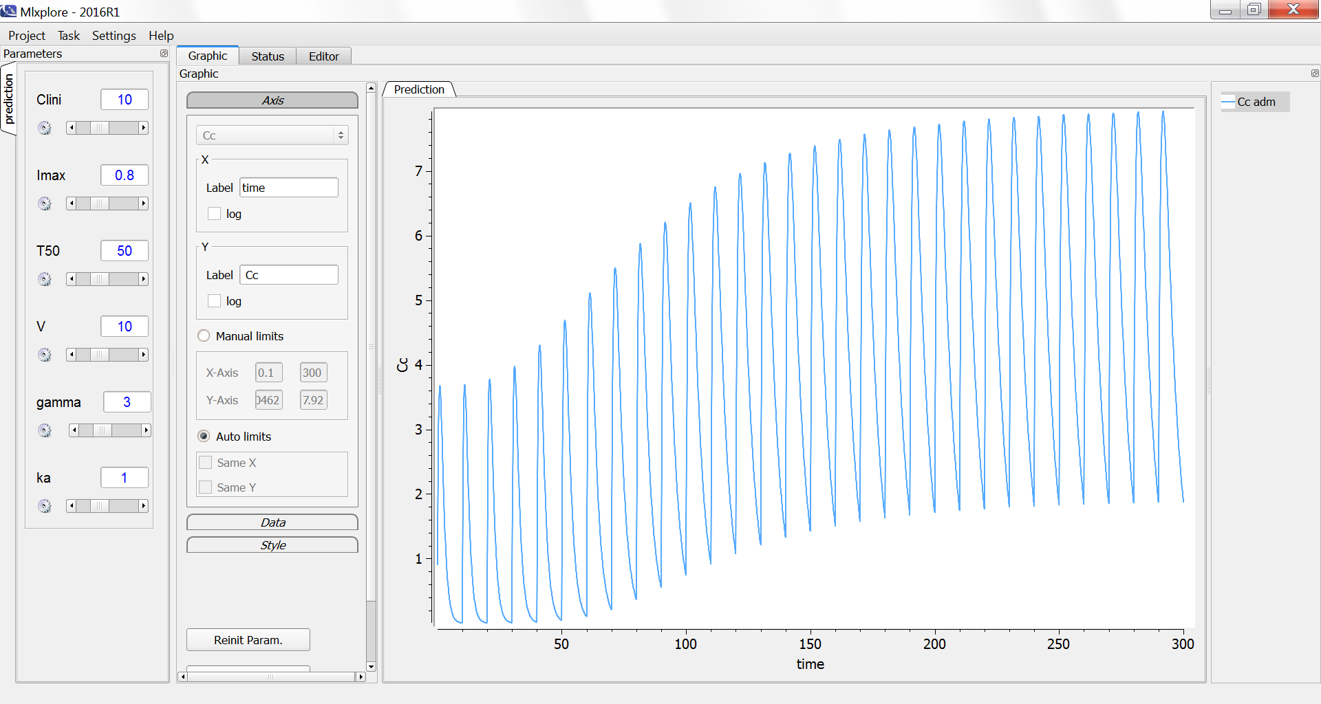
One can compare the original simulation (light blue) with a simulation where the clearance stays constant at 10 L/day (dark blue, with Imax=0):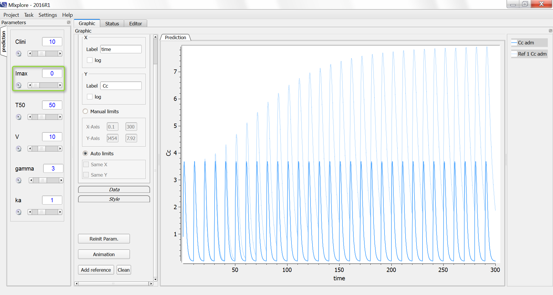
One can also compare the original simulation (light blue) with a simulation where the clearance stays constant at the Clend value 2 L/day (dark blue, with Imax=0 and Clini=2):
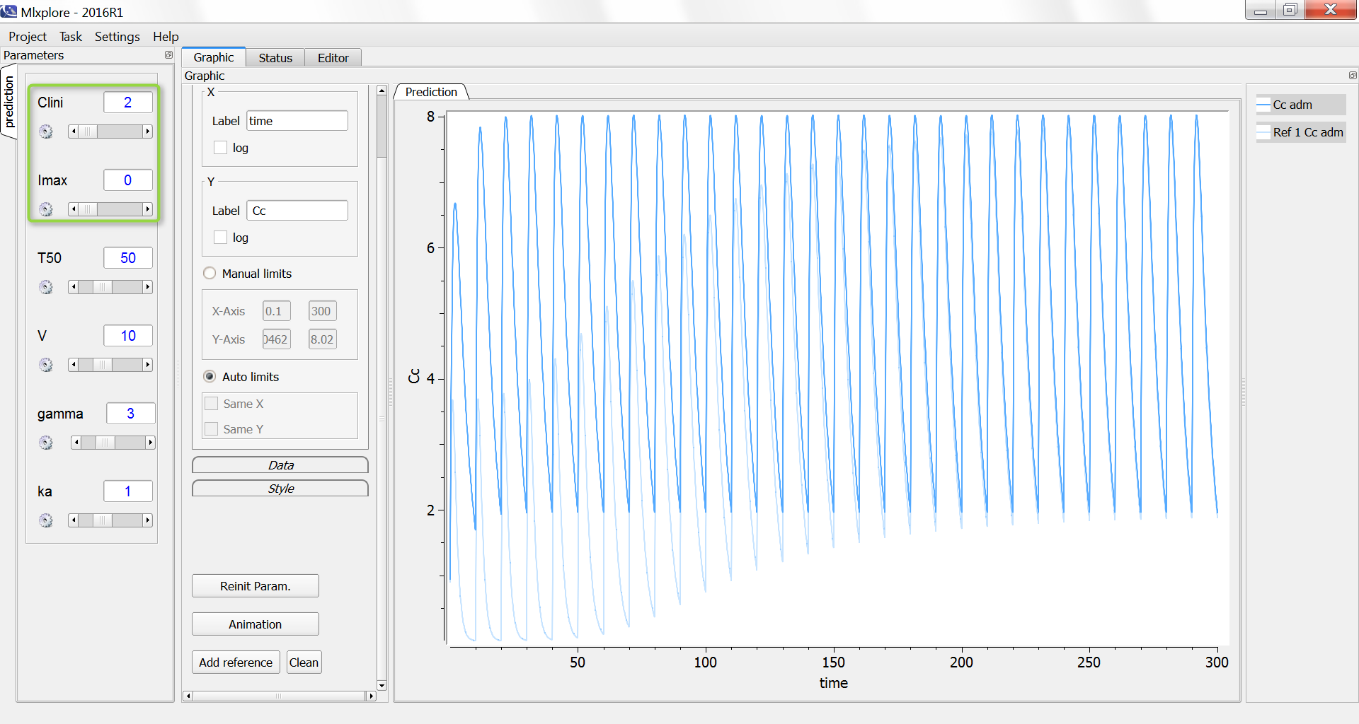
9.8.Auto-induction model
Auto-induction models have been proposed when the drug stimulates its own metabolism, usually via induction of the metabolic enzyme expression. Auto-induction models have for instance been used to describe the pharmacokinetics of Rifampin in Smythe et al. (2012), and of cyclophosphamide in Hassan et al. (1999).
The typical auto-induction model explicitly describes the enzyme level which is modeled using an turnover model with the drug inhibiting the enzyme degradation rate or increasing the enzyme production rate. The enzyme level is then taken into account in the apparent clearance for the drug.
The typical equations read:
 - Cl/V \times Enz \times Ac")
\times Enz")
With In(t) the drug input rate. To avoid unidentifiability issues (i.e the product Cl*Enz0 is identifiable but not Cl and Enz0 separately), the steady-state enzyme level is enforced to 1 which leads to 
Mlxtran code
For a zero-order absorption, the model reads:
[LONGITUDINAL]
input={Tk0, V, Cl, Kenz, IC50}

PK:
depot(target=Ac, Tk0)

EQUATION:
t_0 = 0
Ac_0 = 0
Enz_0 = 1

Cc = Ac/V

ddt_Ac = - Cl/V*Ac*Enz
ddt_Enz = Kenz - Kenz * (1- Cc/(Cc+IC50)) * Enz

OUTPUT:
output = {Cc}
Exploration with Mlxplore
We propose the following Mlxplore script to explore the model interactively:
<MODEL>
[LONGITUDINAL]
input={Tk0, V, Cl, Kenz, IC50}

PK:
depot(target=Ac, Tk0)

EQUATION:
t_0 = 0
Ac_0 = 0
Enz_0 = 1

Cc = Ac/V
ddt_Ac = - Cl/V*Ac*Enz
ddt_Enz = Kenz - Kenz * (1- Cc/(Cc+IC50)) * Enz

<PARAMETER>
Tk0 = 3
V = 15
Cl = 1
Kenz = 0.01
IC50 = 6

<DESIGN>
[ADMINISTRATION]
adm = {time=0:10:500, amount=100}

<OUTPUT>
list={Cc, Enz}
grid=0.1:0.1:300
We obtain the following profile for the drug concentration (blue) and the enzyme (orange). As the drug induces the expression of the enzyme, the clearance of the drug increases leading to lower peak and trough concentrations.
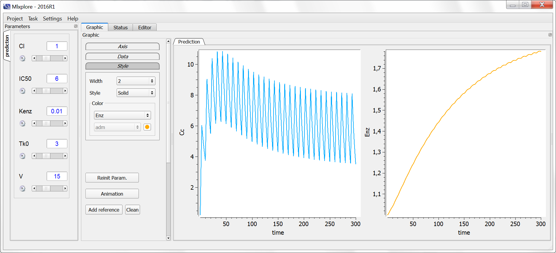
9.9.Enterohepatic circulation model
Enterohepatic circulation (EHC) occurs when drugs circulate from the liver to the bile in the gallbladder, followed by entry into the gut when the bile is released from the gallbladder, and reabsorption from the gut back to the systemic circulation. The presence of EHC results in longer apparent drug half-lives and the appearance of multiple secondary peaks. Various pharmacokinetic models have been used in the literature to describe EHC concentration-time data.
The reference below provides a basic review of the EHC process and modeling strategies implemented to represent EHC.
Mlxtran structural model
We present two examples of EHC models, based on a two-compartments model with iv bolus administration. Both models have been implemented with PK macros.
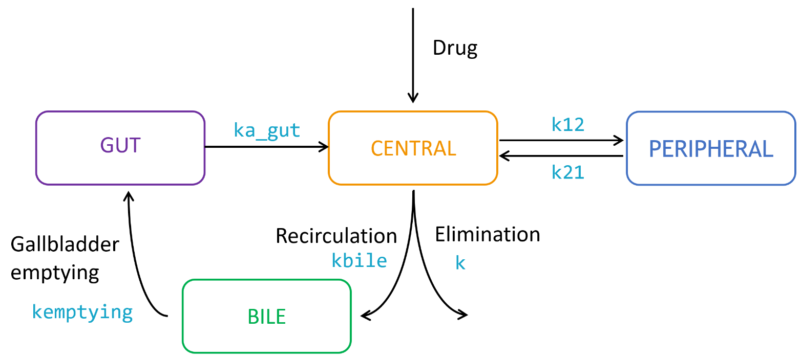
Example with switch function
In the first example, the gallbladder emptying is modelled with a switch function: the emptying rate constant follows a simple piece-wise function, implemented with if/else statements. Hence, gallbladder emptying occurs within time windows, where the rate constant outside these windows is assumed to be zero.
The Mlxtran code for the structural model reads:
[LONGITUDINAL]
input = {V, Cl, Q, V2, kbile, kempt, ka_gut, Tfirst, Tsecond}

PK:
k=Cl/V
k12=Q/V
k21=Q/V2
duration=1
if t>Tfirst & t<Tfirst+duration
kemptying = kempt
elseif t>Tsecond & t<Tsecond+duration
kemptying = kempt
else
kemptying = 0
end

compartment(cmt=1, volume=V, concentration=Cc)
iv(adm=1, cmt=1)
elimination(cmt=1, k)
peripheral(k12, k21)
compartment(cmt=3)
compartment(cmt=4)
transfer(from=1, to=3, kt=kbile)
transfer(from=3, to=4, kt=kemptying)
transfer(from=4, to=1, kt=ka_gut)

OUTPUT:
output = {Cc}
The parameters kbile, kempt and ka_gut describe respectively the transfer rate between the central compartment and the bile, between the bile and the gut, and between the gut and the central compartment.
The parameter kemptying is the rate constant controlling the gallbladder emptying process, and its value changes with time as displayed below:

Here two windows of duration duration=1 have been defined starting at times Tfirst and Tsecond. It is of course possible to extend this model with additional emptying windows, if more than two secondary peaks are noticeable in the data, and to change the value of the parameter duration.
Example with sine function
In the second example, gallbladder emptying is modeled with a sine function, assumed to equal zero outside the gallbladder emptying times. This model accounts for multiple cycles of gallbladder emptying.
The Mlxtran code for the structural model reads:
[LONGITUDINAL]
input = {V, Cl, Q, V2, kbile, kempt, ka_gut, phase, period}

PK:
k=Cl/V
k12=Q/V
k21=Q/V2

kemptying = max(0, kempt * (cos(2*3.14*(t+phase)/period)))

compartment(cmt=1, volume=V, concentration=Cc)
iv(adm=1, cmt=1)
elimination(cmt=1, k)
peripheral(k12, k21)
compartment(cmt=3)
compartment(cmt=4)
transfer(from=1, to=3, kt=kbile)
transfer(from=3, to=1, kt=kemptying)
transfer(from=4, to=1, kt=ka_gut)

OUTPUT:
output = {Cc}
This model assumes fixed intervals between gallbladder release times, with the parameter period defining their frequency. The parameter phase represents the time of the beginning of the first gallbladder release. The value of the parameter kemptying ove time is then:
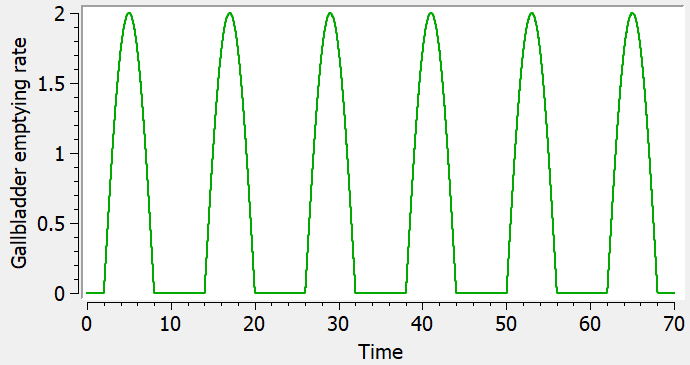
Variation with oral administration
If the drug administration is oral instead of a bolus, the model can be adapted by replacing the macro iv(adm=1, cmt=1) with absorption(adm=1, cmt=1, ka), which defines a first-order absorption with a rate ka. While ka represents the absorption of the drug, ka_gut represents its reabsorption after storage in the gallbladder. These two physiological processes are not strictly equivalent, as the bile stored in the gallbladder is released into the duodenum. Depending on the drug, ka and ka_gut can be set as separate or identical rate constants.
[LONGITUDINAL]
input = {V, ka, Cl, Q, V2, kbile, kempt, ka_gut, phase, period}

PK:
k=Cl/V
k12=Q/V
k21=Q/V2

kemptying = max(0, kempt * (cos(2*3.14*(t+phase)/period)))

compartment(cmt=1, volume=V, concentration=Cc)
absorption(adm=1, cmt=1, ka)
elimination(cmt=1, k)
peripheral(k12, k21)
compartment(cmt=3)
compartment(cmt=4)
transfer(from=1, to=3, kt=kbile)
transfer(from=3, to=1, kt=kemptying)
transfer(from=4, to=1, kt=ka_gut)

OUTPUT:
output = {Cc}
Exploration with Mlxplore
The Mlxplore script below permits to compare the two models with IV bolus, along with the two-compartments model with no EHC.
<MODEL>
[LONGITUDINAL]
input = {V, Cl, Q, V2, kbile, kempt, ka_gut, Tfirst,Tsecond, phase, period}

PK:
k=Cl/V
k12=Q/V
k21=Q/V2

; --- Model with no EHC ---
compartment(cmt=1, volume=V, concentration=Cc_no_EHC)
iv(adm=1, cmt=1)
elimination(cmt=1, k)
peripheral(k12,k21)

; --- EHC model with two constant rate emptying windows ---

if t>Tfirst & t<Tfirst+1
kemptying = kempt
elseif t>Tsecond & t<Tsecond+1
kemptying = kempt
else
kemptying = 0
end

compartment(cmt=3, volume=V, concentration=Cc_EHC_1)
iv(adm=1, cmt=3)
elimination(cmt=3, k)
peripheral(k34=k12, k43=k21)
compartment(cmt=5)
compartment(cmt=6)
transfer(from=3, to=5, kt=kbile)
transfer(from=5, to=6, kt=kemptying)
transfer(from=6, to=3, kt=ka_gut)

; --- EHC model with sine emptying rate ---

kemptying_2 = max(0, kempt * (cos(2*3.14*(t+phase)/period)))

compartment(cmt=7, volume=V, concentration=Cc_EHC_2)
iv(adm=1, cmt=7)
elimination(cmt=7, k)
peripheral(k78=k12, k87=k21)
compartment(cmt=9)
compartment(cmt=10)
transfer(from=7, to=9, kt=kbile)
transfer(from=9, to=10, kt=kemptying_2)
transfer(from=10, to=7, kt=ka_gut)

EQUATION:
odeType=stiff

<PARAMETER>
V=10
Cl=5
Q=2
V2=50
kbile=0.25
kempt=2
ka_gut=0.25
Tfirst = 3
Tsecond=15
phase=7
period=12

<DESIGN>
[ADMINISTRATION]
adm = {type=1, time=0, amount=1000}

<OUTPUT>
list={Cc_no_EHC, Cc_EHC_1, Cc_EHC_2, kemptying, kemptying_2}
grid=0:0.001:70

<RESULTS>
[GRAPHICS]
p1 = {y={Cc_no_EHC, Cc_EHC_1, Cc_EHC_2}, ylabel='Concentration', xlabel='Time'}
p2 = {y={kemptying, kemptying_2}, ylabel='Gallbladder emptying rate', xlabel='Time'}
gridarrange(p1,p2,nb_cols=1)
We obtain the following profiles for the drug concentration in log scale on the top plot below, with no EHC (red), EHC with switch function (blue) and sine function (green). The bottom plot represents the gallbladder emptying rate.
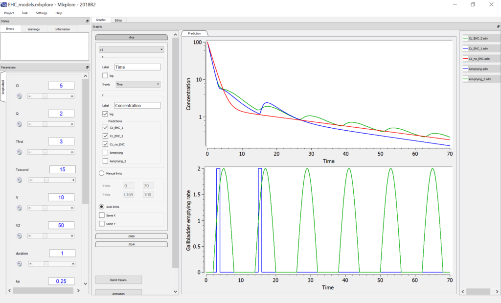
9.10.Models for urine data
When collecting urine data, the urines are collected over several time intervals. For each time interval, the total urine volume and the drug concentration are recorded. The concentration is not relevant by itself, because it strongly depends on the urine volume that itself depend on how much the individual has drunk etc. We are rather interested in the amount of drug excreted in the urine, which is related to the urinary excretion rate.
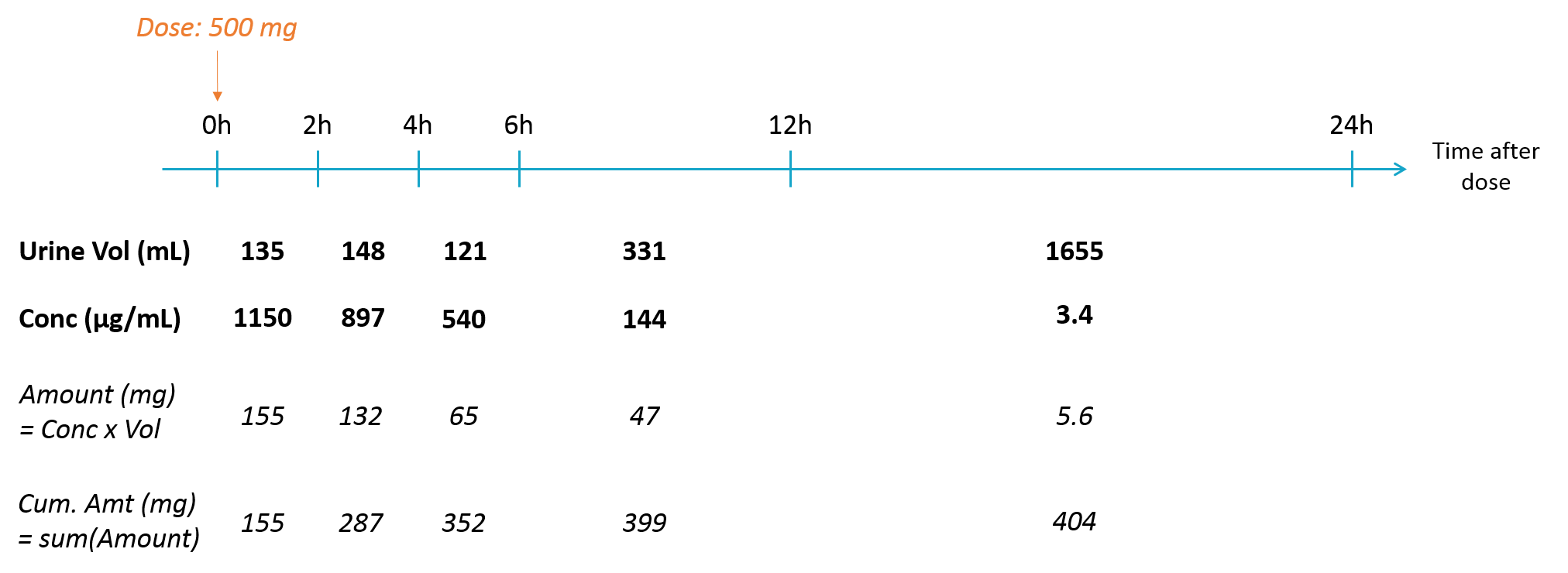
The data can be formatted in several ways:
Using the amount
The amount excreted in each interval can easily be computed by multiplying the concentration and the urine volume. When a new interval starts, the “urine compartment” must be emptied, i.e the variable representing the amount excreted in the urine must be reset to zero. To trigger this reset, pseudo-dose records must be added to the data set. They are distinguished from the true doses by a specific administration identifier (here adm=2) and have an amount of 0. To make sure the reset will happen after the observation, the time of the reset are slightly larger than the time of the observation.
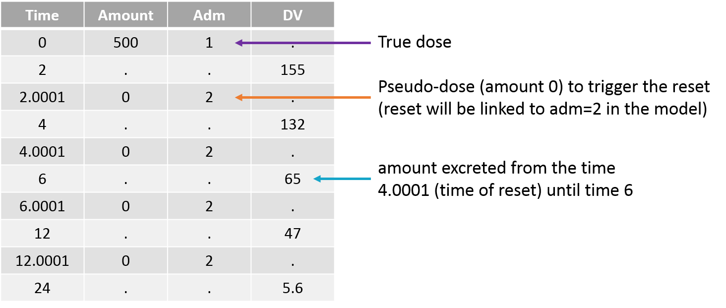
For the model, we will assume that the dose arrives in the central compartment and follows a linear elimination with a rate “k”. A fraction “pu” of the drug is eliminated with the kidney and arrives in the urine. The model is written with ODEs in order to be able to apply the resets. True doses (adm=1 in this example) are applied to the variable Aplasma representing the amount in the plasma (central compartment), while pseudo-doses (adm=2) are linked to the empty() macro which resets its target Aurine (amount excreted in the urine) to zero at the time of the pseudo doses. The amount Aurine is outputted to be mapped to the observations of the data set.
[LONGITUDINAL]
input = {k, pu}

PK:
depot(adm=1, target=Aplasma)
empty(adm=2, target=Aurine)

EQUATION:
t_0 = 0
Aplasma_0 = 0
Aurine_0 = 0

ddt_Aplasma = - k * Aplasma
ddt_Aurine = k * pu * Aplasma

OUTPUT:
output = Aurine
In the “check initial vixed effects” or “individual fits” plot, the resets are clearly visible:

Using the concentration and urine volume
It is also possible to directly use the measured urine volume and drug concentration. The drug concentration is considered as being the observation. To calculate in the predicted drug concentration in the model, the predicted amount excreted in the urine is divided by the urine volume. In order to be passed to the model, the urine volume column in the data set is tagged as regressor. For the parameter estimation in Monolix, only the regressor values on observation lines are important. However, to plot predictions on a regular time grid, Monolix interpolates the regressor values using “Last Observation Carried Forward” and it is necessary to provide a regressor value for the first record (dose or observation line). We thus recommend a provide the urine volume value on all lines.
As when working with the amount, the variable representing the amount excreted in the urine must be reset to zero when a new interval starts. To trigger this reset, pseudo-dose records must be added to the data set. They are distinguished from the true doses by a specific administration identifier (here adm=2) and have an amount of 0. To make sure the reset will happen after the observation, the time of the reset are slightly larger than the time of the observation.
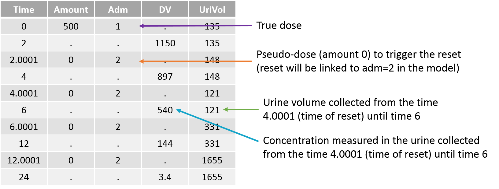
For the model, we will assume that the dose arrives in the central compartment and follows a linear elimination with a rate “k”. A fraction “pu” of the drug is eliminated with the kidney and arrives in the urine. The model is written with ODEs in order to be able to apply the resets. True doses (adm=1 in this example) are applied to the variable Aplasma representing the amount in the plasma (central compartment), while pseudo-doses (adm=2) are linked to the empty() macro which resets its target Aurine (amount excreted in the urine) to zero at the time of the pseudo doses. Before being outputted, the concentration is calculated from the amount in plasma and the urine volume which is indicated as being a regressor and thus read from the data set. Note that the units of the dose, concentration and urine volume must be consistent, or a scaling factor can be added in the model.
[LONGITUDINAL]
input = {k, pu, UriVol}
UriVol = {use=regressor}

PK:
depot(adm=1, target=Aplasma)
empty(adm=2, target=Aurine)

EQUATION:
t_0 = 0
Aplasma_0 = 0
Aurine_0 = 0

ddt_Aplasma = - k * Aplasma
ddt_Aurine = k*pu*Aplasma

Conc = Aurine/UriVol*1000

OUTPUT:
output = Conc
In the “check initial vixed effects” or “individual fits” plot, the resets are clearly visible:
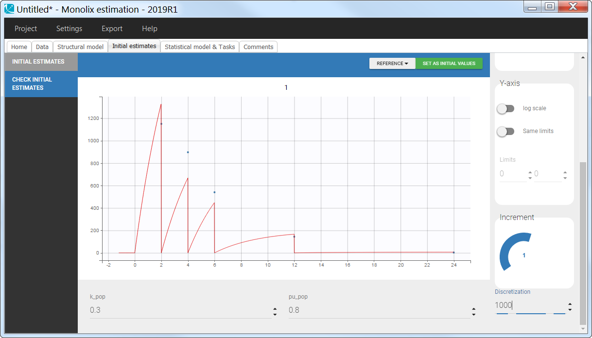
Using the cumulative amount
The cumulative amount can easily be calculated as the sum of the amounts collected from the dose time until the time point of interest. This formatting presents the advantage that no emptying of the urine compartment is necessary. The format of the data set is thus straightforward:
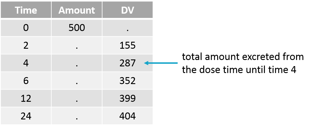
Note that when working with cumulative amounts, if a concentration or urine volume observation is missing, then it is not possible to calculate the cumulative amount for all following time points. Missing information has thus larger consequences than when working with the two other formatting options.
In the model, the cumulative amount is calculated and outputted:
[LONGITUDINAL]
input = {k, pu}

PK:
depot(target = Aplasma)

EQUATION:
t_0 = 0
Aplasma_0 = 0
Aurine_0 = 0

ddt_Aplasma = - k * Aplasma
ddt_Aurine = k*pu*Aplasma

OUTPUT:
output = Aurine
Note that for multiple doses, an emptying of the Aurine variable can be added in the model and in the data set such that the recorded observation represents the cumulative amount from the last dose to the current time.
In the “check initial vixed effects” or “individual fits” plot, the cumulative amount is always increasing (no reset):

9.11.Parent-metabolite model
Parent-metabolite models are common and numerous examples exist in the literature. In Bertrand et al. (2011) for instance, parent-metabolite models of increasing complexity are tested for an antipsychotic agent S33138, using Nonmem and Monolix.
Here we present an example of a simple parent-metabolite model. In the model below, the parent compound is absorbed into a central compartment of volume Vp via a first-order process with rate constant ka, diffuse to a peripheral compartment with rates k12 and k21 and is eliminated with a rate kp. The parent compound is also biotransformed into a metabolite with a first-order rate constant kt. The metabolite is eliminated with a rate constant km. The volume of distribution Vm of the metabolite is not identifiable (see below explanation with Mlxplore) and is thus usually fixed to the volume of the central compartment of the parent (Vm=Vp). 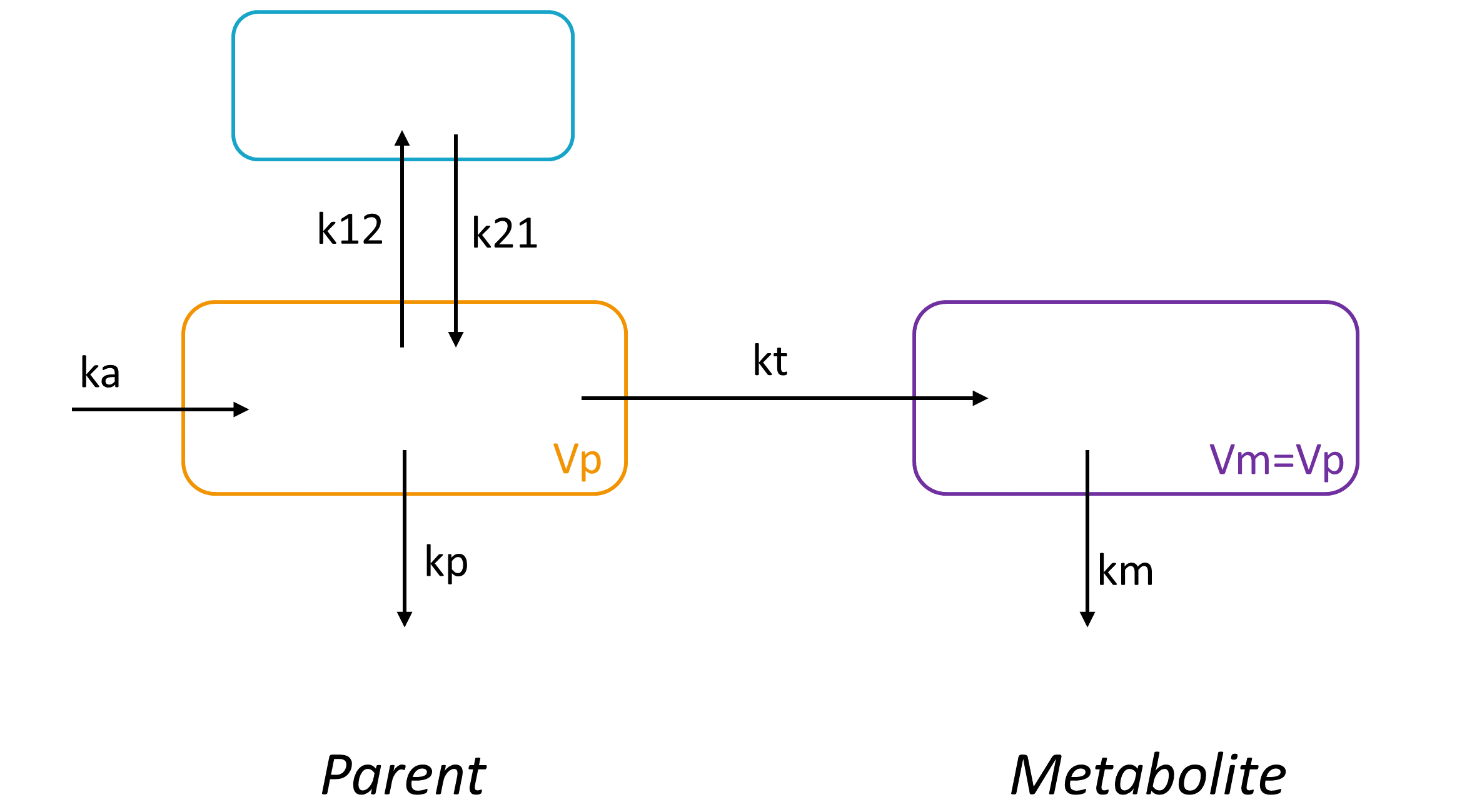
The model can be complexified to take into account a saturation of the biotransformation rate or auto-induction phenomena.
Mlxtran model
The mlxtran code for the structural model reads:
[LONGITUDINAL]
input={ka, Vp, kp, k12, k21, kt, km}

PK:
depot(target=Apc, ka)

EQUATION:
odeType=stiff
t_0 = 0
Apc_0 = 0 ; Apc = amount of parent in central compartment
App_0 = 0 ; App = amount of parent in peripheral compartment
Am_0 = 0  ; Am = amount of metabolite

ddt_Apc = -k12*Apc + k21*App - kp*Apc - kt*Apc
ddt_App = k12*Apc - k21*App
ddt_Am = kt*Apc - km*Am

Cp = Apc/Vp
Cm = Am/Vp

OUTPUT:
output = {Cp, Cm}
The macro depot permits to apply the doses defined in the data set to the ODE system. Here the doses of the data set are applied to the amount of parent in the central compartment via a first-order rate. There is no need to define a depot compartment in the ODE system. All other transfers are defined in the ODE system. The first output of the list (Cp) will be matched to the data with lowest OBSERVATION ID tag (OBSERVATION ID = 1 usually) and the second output (Cm) will be matched to the data with the second OBSERVATION ID tag (OBSERVATION ID = 2 usually). The odeType=stiff line permits to choose an ODE solver designed for stiff systems.
Unidentifiability of Vm explored with Mlxplore
Except when the metabolite has also been administrated, the volume of distribution Vm of the metabolite is not identifiable for the following reason: an increase of Vm can be compensated by a decrease in the biotransformation rate kt, which itself can be compensated by an adjustment of the elimination rate of the parent kp. Note that the disappearance of the parent (via elimination or biotransformation) is driven by ktot=kp+kt and that any combination of kt and kp values that leads to the same ktot will keep the parent concentration-time profile unchanged.
To better grasp this unidentifiability, we propose the following Mlxplore script, where Vm is considered a separate parameter:
<MODEL>
[LONGITUDINAL]
input={ka, Vp, kp, k12, k21, kt, Vm, km}

PK:
depot(target=Apc, ka)

EQUATION:
odeType=stiff
t_0 = 0
Apc_0 = 0
App_0 = 0
Am_0 = 0

ddt_Apc = -k12*Apc + k21*App - kp*Apc - kt*Apc
ddt_App = k12*Apc - k21*App
ddt_Am = kt*Apc - km*Am

Cp = Apc/Vp
Cm = Am/Vm

<PARAMETER>
ka = 1
Vp = 10
kp = 0.1
k12 = 0.05
k21 = 0.05
kt = 0.02
Vm = 15
km = 0.01

<DESIGN>
[ADMINISTRATION]
adm = {time=0, amount=100}

<OUTPUT>
list={Cp, Cm}
grid=0.1:0.1:150
We can then test different values of Vm, kt and kp. The following sets of values (Vm=15, kt=0.02, kp=0.1) and (Vm=30, kt=0.04, kp=0.08) lead to exactly the same prediction for both the parent and the metabolite, highlighting the unidentifiability. One of these 3 parameters must therefore be fixed, the most common choice is to fix Vm to the value of Vp.
9.12.Mechanistic QSP model of a PSCK9 inhibitor
| Here we give an example of QSP model for RG7652, published in Gadkar et al., CPT Pharmacometrics Syst. Pharmacol. 3, (2014) and translated in Mlxtran. A Monolix project estimating this model on phase I clinical data extracted from the plots from the same publication can be downloaded here.
Compared to PK/PD models, QSP models incorporate more mechanistic details and model entities which have not been measured experimentally. By putting more emphasis on the biological relevance, QSP models are believed to be more capable of extrapolating from preclinical to clinical or from healthy volunteers to patients.
The poster given on the right compares this QSP model to a typical PK/PD model |
|
Anti-PCSK9 mAb for cholesterol lowering
RG7652 [1] is a fully human monoclonal antibody antagonizing PSCK9 activity. It is developed as cholesterol (LDLc) lowering therapy and can be given in patients already treated with statins.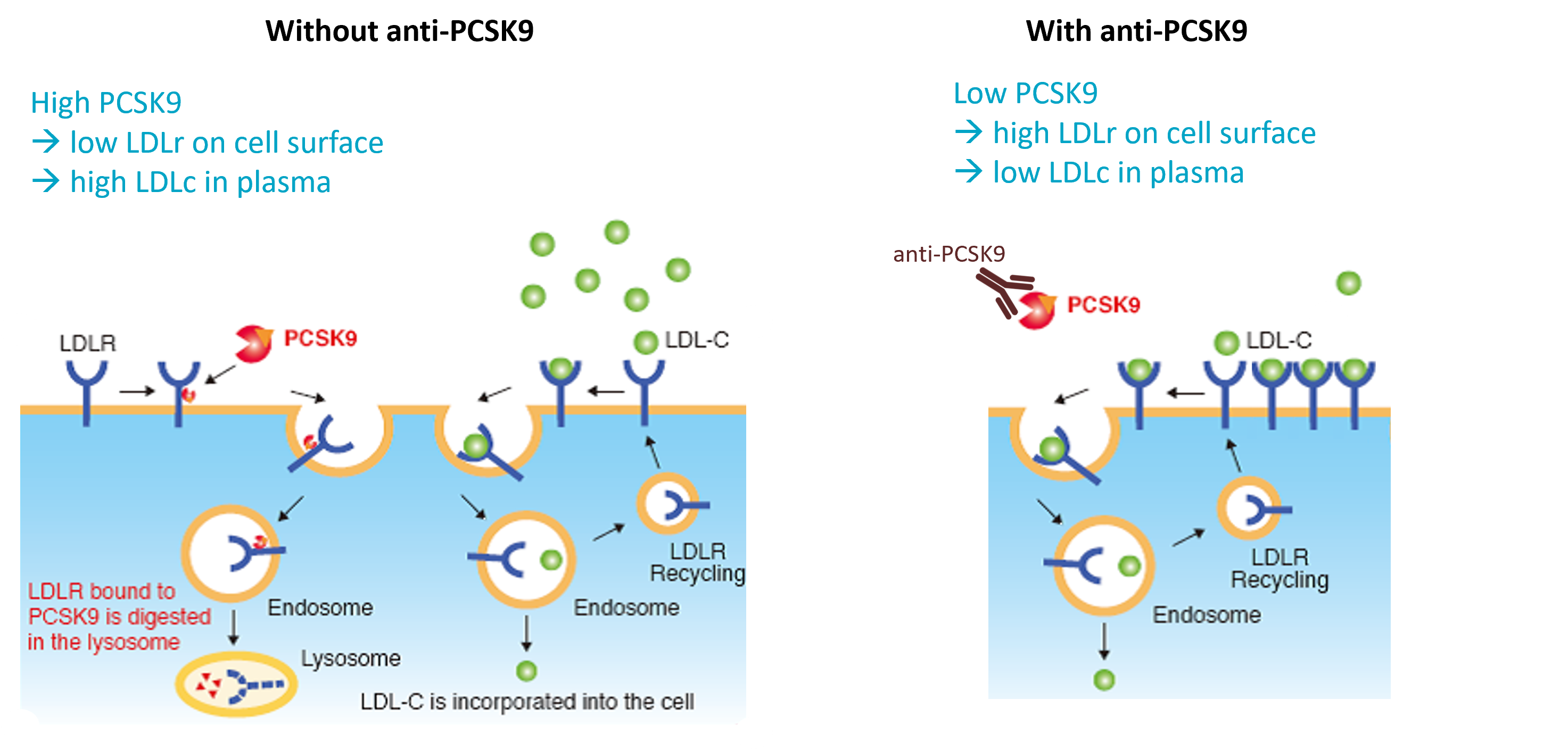
QSP model
The structural model (full text given below) is composed of six ODEs and 21 parameters. The modeled entities are:
- L: Drug
- P: Drug-PCSK9 complex
- PCSK9: Circulating PCSK9
- LDLr: LDL receptor
- LDLc: LDL cholesterol
- HepCh: Hepatic cholesterol
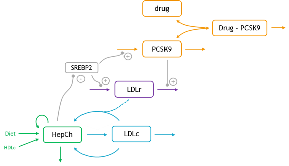
The model allows to investigate several questions by simulation, such as statin effect or the response of patients with familial hypercholesterolemia (FH).
Simulating statin effect
Statins induce SREBP2 which increases PCSK9 and LDLr levels (via increased synthesis), increased LDLr levels and may also decrease hepatic cholesterol synthesis. Thus the effect of statin can be implemented with:
- ksynPCSK9 increased, kdegPCSK9 same (but LDLr increased) => PCSK9 increased
- ksynLDLr increased, kdegLDLr same (but PCSK9 increased) => LDLr increased
- ksynLDLc same, kdegLDLc same but LDLr increased => LDLc decreased
Response of patients with familial hypercholesterolemia
These patients have a low concentrations of LDLr receptor due to mutations.
Full structural model
[LONGITUDINAL]
input = {ka, V, Cl, kint, KD, S_diet, f_diet_abs,S_HepCh_syn, f_HepCh_statin, k_HepCh_loss, k_LDL_syn, Ch_LDLparticle, k_LDLc_clr1, f_LDLcHep_clr, k_LDLc_clr2, k_HDLc_clr, Vblood, LDLr0, k_LDLr_deg, k_PCSK9_deg, k_PCSK9_syn}


PK:
MW = 150
depot(target=L, ka, p=1/V * 1000/MW)
; dose in mg
; L in nmol/L
; V in L

EQUATION:
odeType=stiff

t_0 = -100
L_0 = 0
P_0 = 0
HepCh_0 = 6000
LDLc_0 = 160
LDLr_0 = 1
PCSK9_0 = k_PCSK9_syn/k_PCSK9_deg
k_LDLr_syn = LDLr0 * k_LDLr_deg

HDLc = 50
kel = Cl/V
kon = 10
koff = KD*kon

; ======== effect of HepCh on PCSK9
maxSREBP2level = 2
minSREBP2level = 0
HepChref = 6000
expT=3.97865*3^-0.995 ; This is fitted to give 99% output at the extreme of the range specified

f_HepCh_reg=( minSREBP2level - maxSREBP2level ) * (HepCh^expT/(HepCh^expT+HepChref^expT)) + maxSREBP2level
SREBP2 = f_HepCh_reg

; ======== effect of PCSK9 on LDLr degradation
nM2ngPermL=74
pcsk9_on_LDLr = 0.75
Baselinepcsk9 = 281.94
pcsk9_on_LDLr_range = 650

expT=3.97865*2^-0.995
Xmod=10^( 2*(PCSK9*nM2ngPermL-(Baselinepcsk9-pcsk9_on_LDLr_range/2))/pcsk9_on_LDLr_range -1 )
Xmodic50=10^( 2*(Baselinepcsk9-(Baselinepcsk9-pcsk9_on_LDLr_range/2))/pcsk9_on_LDLr_range -1 )
f_PCSK9_degLDLr = 2*pcsk9_on_LDLr * (Xmod^expT/(Xmod^expT+Xmodic50^expT)) + (1-pcsk9_on_LDLr)


; ======== effect of SREBL2 on LDLr
VmaxUpLDLr=3
KmUpLDLr=1.5
VmaxDownLDLr=0.7
KmDownLDLr=0.5

if SREBP2>1
f_SREBP2_regLDLr = 1+ (VmaxUpLDLr-1) * (SREBP2-1)/((SREBP2-1)+(KmUpLDLr-1))
else
f_SREBP2_regLDLr = 1 - VmaxDownLDLr * (1-SREBP2)/((1-SREBP2)+KmDownLDLr)
end

; ======== effect of SREBL2 on PCSK9
VmaxUpPCSK9=2
KmUpPCSK9=1.5
VmaxDownPCSK9=0.7
KmDownPCSK9=0.5

if SREBP2>1
f_SREBP2_regPCSK9 = 1+ (VmaxUpPCSK9-1) * (SREBP2-1)/((SREBP2-1)+(KmUpPCSK9-1))
else
f_SREBP2_regPCSK9 = 1 - VmaxDownPCSK9 * (1-SREBP2)/((1-SREBP2)+KmDownPCSK9)
end

; ========= ODEs
ddt_HepCh = f_diet_abs * S_diet + f_HepCh_statin * S_HepCh_syn - k_HepCh_loss * HepCh - k_LDL_syn * Ch_LDLparticle * Vblood * HepCh + f_LDLcHep_clr * k_LDLc_clr1 *Vblood * LDLc * LDLr + f_LDLcHep_clr * k_LDLc_clr2 * Vblood * LDLc + f_LDLcHep_clr * k_HDLc_clr * Vblood * HDLc

ddt_LDLc = k_LDL_syn * Ch_LDLparticle * HepCh - k_LDLc_clr1 * LDLc * LDLr - k_LDLc_clr2 * LDLc

ddt_LDLr = k_LDLr_syn * f_SREBP2_regLDLr - k_LDLr_deg * LDLr * f_PCSK9_degLDLr

ddt_PCSK9 = k_PCSK9_syn * f_SREBP2_regPCSK9 - k_PCSK9_deg * PCSK9 - kon*L*PCSK9 + koff*P

ddt_P = kon*L*PCSK9 - koff*P - kint*P

ddt_L = -kel*L - kon*L*PCSK9 + koff*P

Ltot = L+P
Rtot = PCSK9+P
LDLc_change = LDLc/160*100

PCSK9_ngmL = PCSK9*74 ; from nmol/L to ng/mL
LDLc_mgdL = LDLc

OUTPUT:
output={Ltot, Rtot, LDLc_change}
9.13.Friberg model for myelosuppression
The Friberg model is a semi-mechanistic pharmacodynamic model describing chemotherapy-induced myelosuppression. It has been originally developed to describe leukocyte and neutrophil data after administration of docetaxel, paclitaxel, etoposide, DMDC and irinotecan and vinflunine in Friberg et al. (2002), and has been reused in many other publications since.
Model description
The model consists of a proliferating compartment that is sensitive to drugs, three transit compartments that represent maturation, and a compartment of circulating blood cells. The parameterization is parsimonious (initial circulating concentration, mean transit time and a feedback parameter), well suited for sparse data. The drug effect can be implemented as a linear function or with an Emax model, as shown below.

The PK part of the model is in this example a (ka,V,Cl) model but can be replaced by any other PK model. PK parameters can either be estimated (as below) or read from the data set (uncomment the three lines below the input line to consider the PK parameters as regressors).
Mlxtran model code
The model code can be downloaded here.
DESCRIPTION:
PD = Friberg et al (2002) 'Model of Chemotherapy-Induced Myelosuppression with Parameter Consistency Across Drugs', Journal of Clinical Oncology 20:4713-4721

[LONGITUDINAL]
input = {ka, V, Cl, Circ0, MTT, gam, Emax, EC50}
; ka = {use=regressor}
; V  = {use=regressor}
; Cl = {use=regressor}

EQUATION:
odeType=stiff
; PK model
Cc = pkmodel(ka, V, Cl)

; parameter transformations
n = 3
ktr = (n+1)/MTT
kprol = ktr
kcirc = ktr

; drug effect
Edrug = Emax * Cc/(EC50 + Cc)

; initial values
t_0 = 0
Prol_0 = Circ0
T1_0 = Circ0
T2_0 = Circ0
T3_0 = Circ0
Circ_0 = Circ0

;ODEs for the response
ddt_Prol = kprol*Prol*(1-Edrug)*(Circ0/Circ)^gam - ktr*Prol
ddt_T1 = ktr*Prol - ktr*T1
ddt_T2= ktr*T1 - ktr*T2
ddt_T3 = ktr*T2 - ktr*T3
ddt_Circ = ktr*T3 - kcirc*Circ

OUTPUT:
output = {Cc, Circ}
In the Monolix GUI, a lognormal distribution can be chosen for Circ0, MTT, gam and EC50, and a logit distribution for Emax to ensure that (1-Edrug) stays always positive. It is common to remove the random effects on gam.
9.14.K-PD models
Usual PK-PD models describe the relationships between dose regimens, drug concentration and effect (or response). They are applied when both the drug concentration and the effect can be measured. However situations exist where the concentration PK data is not available. This may for instance be the case for phase III clinical trials or pediatric studies. In this case K-PD models can be used: the drug concentration-effect relationship model is kept, but the (unobserved) PK profile is assumed to have a simple shape. In comparison to dose-response studies which directly link the (constant) dose to the PD response, K-PD models permit to capture PD profile that varies over time as a consequence of the underlying time-varying PK profile.
Although not being the first published example of K-PD model, the usual reference is:
Mlxtran code for K-PD models
The effect of the drug on the response can be as diverse as presented in the indirect response models and direct response models examples. We here focus on the case of an indirect response where the drug decreases the response production rate.
Formulation by Jacqmin et al.
The authors in Jacqmin et al. describe the model in the following way: “A virtual compartment representing the biophase in which the concentration is in equilibrium with the observed effect is used to extract the (pharmaco)kinetic component from the pharmacodynamic data alone. Parameters of this model are the elimination rate constant from the virtual compartment (KDE), which describes the equilibrium between the rate of dose administration and the observed effect, and the second parameter, named EDK50 which is the apparent in vivo potency of the drug at steady state.
The equations read:


 - K_D R")
with A the drug amount, R the response, KDE the drug elimination rate, Ks the response synthesis rate, Kd the response disappearance rate constant. EDK50 represents the potency of the drug and also corresponds to EDK50 constant corresponds to the product of the EC50 and the clearance.
The corresponding Mlxtran code is:
[LONGITUDINAL]
input={Ks,Kd,KDE,EDK50}

PK:
depot(target=A)

EQUATION:
; initialization
t_0 = 0
A_0 = 0
R_0 = Ks/Kd

; ODEs
ddt_A = - KDE*A
ddt_R = Ks * (1 - (KDE*A)/(EDK50 + (KDE*A))) - Kd*R

OUTPUT:
output = {R}
Note that the only output is the response R, as only the response has been measured and recorded in the data set.
Alternative formulation
For some applications, the interpretation of the parameters of the Jacqmin model may be difficult. It is also unusual the consider that it is the rate at which the drug disappear (IR) that drives the effect on the response. We thus propose an alternative formulation of the same model.
We start by writing the model using the usual (and physiologically relevant) effect of the drug concentration on the response:

 - K_D R")
This set of equations can be rewritten into:
 - K_D R")
using the fact that 


We thus introduce 
 - K_D R")
The parameter 
The mlxtran model reads:
[LONGITUDINAL]
input={Ks,Kd,KDE,A50}

PK:
depot(target=A)

EQUATION:
; initialization
t_0 = 0
A_0 = 0
R_0 = Ks/Kd

; ODEs
ddt_A = - KDE*A
ddt_R = Ks * (1 - A/(A50 + A) ) - Kd*R

OUTPUT:
output = {R}
The model can also be written using macros for the (P)K part. When macros are used, the PK part of the model will be calculated using the analytical solution while the PD part will be solved using the ODE solver.
[LONGITUDINAL]
input={Ks,Kd,KDE,A50}

PK:
compartment(cmt=1, amount=A)
iv(cmt=1)
elimination(cmt=1, k=KDE)

EQUATION:
; initialization
t_0 = 0
R_0 = Ks/Kd

; ODEs
ddt_R = Ks * (1 - A/(A50 + A) ) - Kd*R

OUTPUT:
output = {R}
Extensions
If data is sufficient to allow for the estimation of the additional parameters, the model can be extended, for instance in the following directions:
- more complex profile for the drug concentration, for example with a first-order input rate. In this case, the additional input arguments can be directly given in the depot macro.
- sigmoïdal Emax or Imax model with a hill exponent
- Emax or Imax value different from one
The model can also be adapted to consider K-PK models, where two drugs interact and only one of the two is measured.
Simplifications
The use of an Emax or Imax model is only suited if the dose range is sufficiently large to cover both the linear and saturating part of the Michaelis-Menten curve. If concentrations are always smaller than the EC50, the model simplifies to:
 - K_D R")
test
Exploration of the unidentifiability of the drug volume of distribution with Mlxplore
In the section above, we have seen why the volume of distribution is not identifiable from a mathematical point of view. In this section, we explore this unidentifiability interactively with Mlxplore.
The following Mlxplore script defines the model (using the alternative formulation and including the volume), the reference parameter values, an arbitrary dose for A and the simulation output:
<MODEL>
[LONGITUDINAL]
input={Ks,Kd,KDE,IC50,V}

EQUATION:
; initialization
t_0 = 0
A_0 = 0
R_0 = Ks/Kd

; ODEs
ddt_A = - KDE*A
CA = A/V
ddt_R = Ks * (1 - CA/(IC50 + CA) ) - Kd*R

OUTPUT:
output = {R}

<PARAMETER>
KDE=0.5
IC50=50
Ks=0.1
Kd = 0.01
V=1

<DESIGN>
[ADMINISTRATION]
adm={amount=100, time=0, target=A}

<OUTPUT>
list={A,CA,R}
grid=-1:0.1:50

<RESULTS>
[GRAPHICS]
p1 = {y=A, ylabel='Assumed drug amount', xlabel='Time'}
p2 = {y=CA, ylabel='Assumed drug concentration', xlabel='Time'}
p3 = {y=R, ylabel='Indirect response', xlabel='Time'}
Using the sliders to play with the parameter values, it can easily be seen that several sets of parameters lead to the same prediction for the response, compare for instance (V=1,IC50=50) and (V=2,IC50=25). The drug concentration on the opposite is not the same, but as it is not measured, it cannot help in identifying uniquely V and IC50.
In the figure below, we see the drug amount in blue, the drug concentration in orange and the response in green. The first set of parameters is displayed in light colors and the second set in darker colors.

Comparison of dose-response and K-PD approaches for the indirect model with Mlxplore
When an indirect response model is used, it is also common to do a dose-response approach, where the response is directly influenced by the dose instead of the drug concentration as in the K-PD approach. In this section, we will compare the two methods and see when one or the other is more appropriate.
The equation for the dose-response approach is:
 - K_D R")
As a reminder, the equations for the K-PD model are:
We first note that the dose-response model has 3 parameters (


The Mlxplore script below permits to compare the two models. The reserved keyword amtDose is used to recover the dose defined in the [ADMINISTRATION] block.
<MODEL>
[LONGITUDINAL]
input={KDE, Ks, Kd, A50, D50}

EQUATION:
; initialization
t_0 = 0
A_0 = 0
Ed_0 = Ks/Kd
Ea_0 = Ks/Kd

; indirect model with Dose (dose-response)
ddt_Ed = Ks * (1 - amtDose / (amtDose + D50)) - Kd * Ed

; indirect with K-PD
ddt_A = - KDE * A
ddt_Ea = Ks * (1 - A / (A + A50)) - Kd * Ea

<PARAMETER>
KDE=0.2
A50=5
D50=150
Ks=0.1
Kd=0.05

<DESIGN>
[ADMINISTRATION]
adm_singledose={amount=100, time=0, target=A}
;adm_multipledose1={amount=100, time=0:50:1000, target=A}
;adm_multipledose2={amount=200, time=1050:50:1500, target=A}

[TREATMENT]
trt_singledose = {adm_singledose}
;trt_multipledose = {adm_multipledose1,adm_multipledose2}

<OUTPUT>
list={Ed,Ea}
grid=-3:0.1:150
;grid=-1:0.1:1500

<RESULTS>
[GRAPHICS]
p1 = {y=Ed, ylabel='Indirect response with Dose', xlabel='Time'}
p2 = {y=Ea, ylabel='Indirect response with K-PD', xlabel='Time'}
In the simulation below, the response of the dose-response model (orange) and of the K-PD model (blue) for a single dose are plotted. The two profiles differ clearly and only the K-PD model is able to capture the transient effect of the drug. If PD data is recorded densely after a dose, a K-PD is usually more appropriate to describe the data.
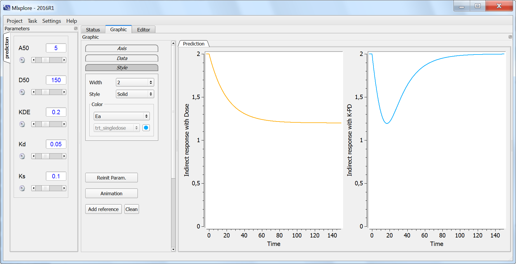
On the next simulation, the two models (dose-response in orange and K-PD in blue) are compared in the case of multiple doses. Note that at time 1000 the initial dose is increased by a factor 2. The only difference between the two models is that the K-PD model captures the small inter-dose variations, while the dose-response model does not. If the PD data is sparse, the dose-response model is usually sufficient. If the K-PD model is used, the KDE parameter may not be identifiable.
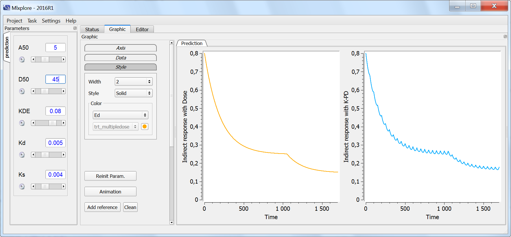
Data set formatting
The data set associated with K-PD models usually has one type of administration (administration of drug A) and one type of measurement (measurement of the response R). Below we show a data set extract:

The dose lines will be associated to the drug A via the depot statement depot(target=A). The measurement lines will be associated to the response R via the output statement output={R}. As there is only one type of administration and one type of observations, there is no need for the ADM and YTYPE columns.
9.15.Lifespan based indirect response models
Lifespan based indirect response (LIDR) models have originally been proposed in the field of hematology. The population of cells are described by cell production and cell degradation. The main assumption of LIDR models is that a cell dies when its lifespan expires. This implies that the cell degradation rate is equal to the cell production rate delayed by the lifespan. This assumption differs from classical indirect response model where the cell (or response) degradation is proportional to the cell number (first-order process), independently of the production rate or the lifespan.
LIDR models have been reviewed in detail in:
The implementation of LIDR model makes use of delayed differential equations, which can easily be solved in the MonolixSuite using the delayed differential equation solver. In the following, we will consider a drug with simple exponential decay after a bolus administration and a response R, which can for instance be the number of blood cells.
Mlxtran code for LIDR models
LIDR model for drugs affecting the production rate of the response
In this model, the drug affects the response via an Imax model on the production rate. The equation for the response is:
}{IC50+C(t)} \right) - k_{in} \left( 1 \pm I_{max} \frac{C(t-T_R)}{IC50+C(t-T_R)} \right)")
where + would be used if the drug increases the production rate and – if it decreases it. Notice that the degradation rate is simply the production rate delayed by the lifespan 
")
delay(C,TR) which means that we use the value of the concentration C delayed by time
Note that the delay function makes use of the DDE solver, which is slower than the ODE solver. This video presents an alternative implementation using ODEs only, which leads to greatly shorter run times.
The mlxtran code reads (for the inhibition case):
[LONGITUDINAL]
input={V, k, kin, Imax, IC50, TR}

PK:
depot(target=Ac)

EQUATION:
t_0 = 0
Ac_0 = 0
R_0 = kin * TR

Cc = Ac/V
ddt_Ac = -k*Ac
ddt_R = kin*(1 - Imax *Cc/(Cc+IC50)) - kin*(1 - Imax *delay(Ac,TR)/(delay(Ac,TR)+IC50*V))

OUTPUT:
output = {Cc, R}
As usual, the depot macro permits to link the doses defined in the data set to the DDEs system.
In the model formulation above, it is assumed that both the drug concentration Cc and the response R are recorded in the data set. If only R is observed, the output line should be changed to output= {R}. Note that if the concentration Cc is not observed, it is not possible to identify both V and IC50. The value of V can then be fixed. Alternatively, the K-PD model can be reformulated as in Jacqmin et al. (2007).
In the delay macro, it is mandatory to use an ODE variable. We thus use Ac rather than Cc and divide by the volume V outside of the delay macro.
For a drug inhibiting the production rate, the typical response shape is the following (darker colors indicate larger drug amounts). The response start to change from baseline at time 0 and is maximal at time 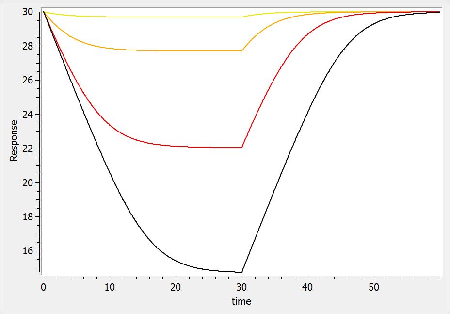
If the drug would increase the production rate instead of decreasing it, the response would increase over time before recovering its basal level: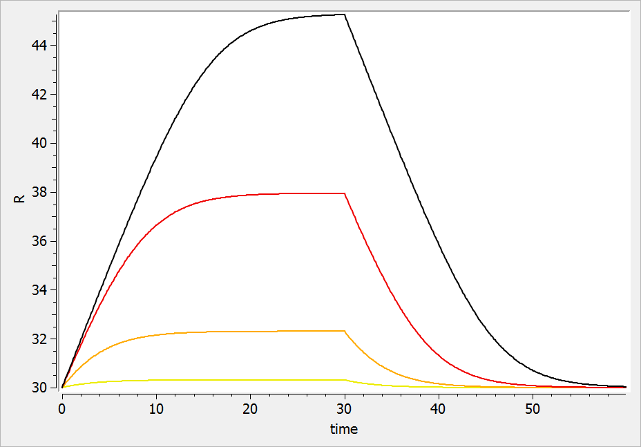
LIDR model for drugs affecting the cell lifespan distribution
This model assumes that initially the lifespan is 
The equation for the response is:
}{IC50+C(t-T_R)} \right) - k_{in} \left( I_{max} \frac{C(t-T_D)}{IC50+C(t-T_D)} \right)")
The mlxtran code reads:
[LONGITUDINAL]
input={V, k, kin, Imax, IC50, TR, TD}

PK:
depot(target=Ac)

EQUATION:
t_0 = 0
Ac_0 = 0
R_0 = kin * TR

Cc = Ac/V
ddt_Ac = -k*Ac
ddt_R = kin - kin*(1 - Imax *delay(Ac,TR)/(delay(Ac,TR)+IC50*V)) - kin*(Imax *delay(Ac,TD)/(delay(Ac,TD)+IC50*V))

OUTPUT:
output = {Cc, R}
For a drug reducing the lifespan from 

")
")
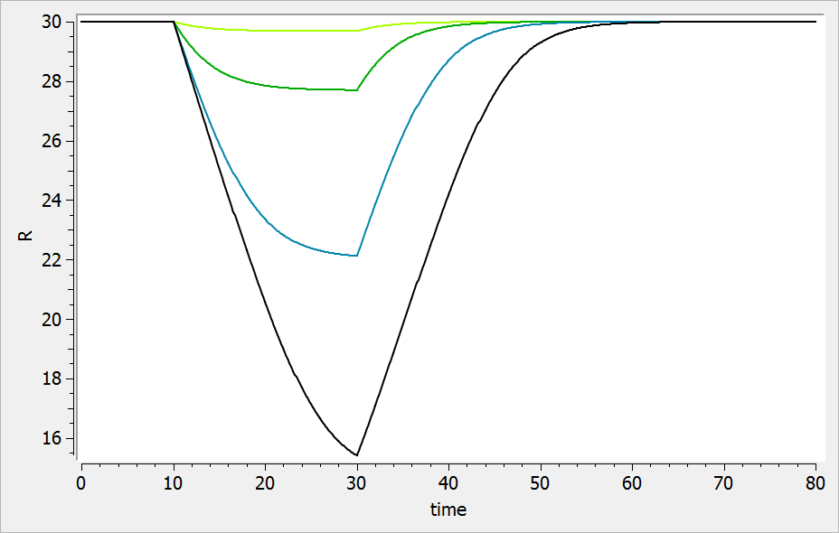
If the drug would increase the lifespan (i.e 
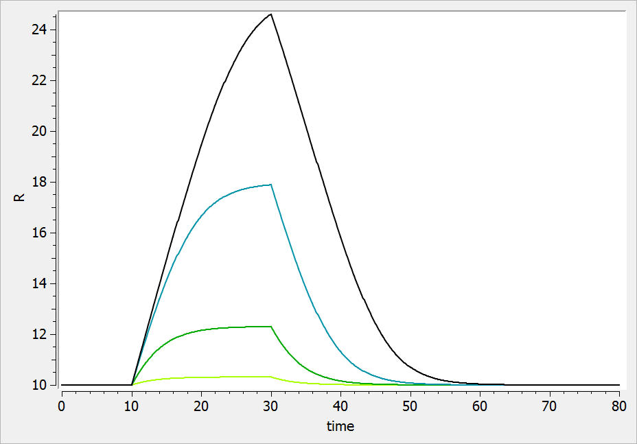
LIDR model with a precursor pool
In this model we assume that the drug effects a precursor pool, which matures into the main pool represented by the response R. Interestingly, it is not necessary to solve the equation for the precursor, only the equation for the response R is needed:
}{IC50+C(t-T_P)} \right) - k_{in} \left( 1 \pm I_{max} \frac{C(t-T_P-T_R)}{IC50+C(t-T_P-T_R)} \right)")
where + is used if the drug increases the precursor production rate and – if it decreases it. 
The mlxtran code reads:
[LONGITUDINAL]
input={V, k, kin, Imax, IC50, TR, TP}

PK:
depot(target=Ac)

EQUATION:
t_0 = 0
Ac_0 = 0
R_0 = kin * TR

Cc = Ac/V
ddt_Ac = -k*Ac
ddt_R = kin*(1 - Imax *delay(Ac,TP)/(delay(Ac,TP)+IC50*V)) - kin*(1 - Imax *delay(Ac,TP+TR)/(delay(Ac,TP+TR)+IC50*V))

OUTPUT:
output= {Cc, R}
The typical response-time curve is displayed below for the case where the drug inhibits the precursor production. The response start to change at time 
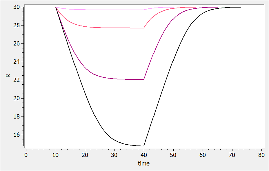
If the drug increases the precursor production, we obtain: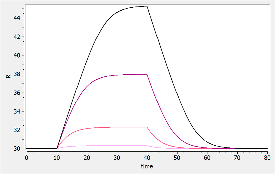
Exploration of indirect model and LIDR model differences with Mlxplore
We explore the differences between:
- the LIDR model
- the indirect response model
In both models, we assume that the drug inhibits the response production rate. Yet, in the LIDR model, the response degradation rate is equal to the production rate delayed by the lifespan. On the opposite, in the indirect response model, the response degradation rate is proportional to the response magnitude.
In the Mlxplore code below, we have implemented both models with same PK parameters and same production rate kin. To set the same baseline for the two responses, we have assume that the value of the degradation rate for the indirect response model kout is the inverse of the lifespan of the LIDR model.
<MODEL>
[LONGITUDINAL]
input={V, k, kin, Imax, IC50, TR}

PK:
depot(target=Ac)

EQUATION:
; initial values
kout = 1/TR ; to ensure same baseline levels for both
t_0 = 0
Ac_0 = 0
RLIDR_0 = kin * TR
Rind_0 = kin/kout

; drug equations
Cc = Ac/V
ddt_Ac = -k*Ac

; LIDR model
ddt_RLIDR = kin*(1 - Imax *Cc/(Cc+IC50)) - kin*(1 - Imax *delay(Ac,TR)/(delay(Ac,TR)+IC50*V))

; indirect response model
ddt_Rind = kin*(1 - Imax *Cc/(Cc+IC50)) - kout*Rind

<PARAMETER>
V = 10
k = 0.3
kin = 1
Imax = 1
IC50 = 10
TR = 30

<DESIGN>
[ADMINISTRATION]
adm10 = {time=0, amount = 10}
adm100 = {time=0, amount = 100}
adm1000 = {time=0, amount = 1000}
adm10000 = {time=0, amount = 10000}

<OUTPUT>
list={RLIDR,Rind}
grid=0:0.1:60
In the figure below, one can observe how the response for the LIDR model (left plot) plateaus, which is not the case for the indirect model response (right plot). In addition, the peak response time is the same for all drug concentration in the LIDR model but not the in indirect response model. Finally, the relationship between the drug concentration and the extend of the response also differ between the two models.
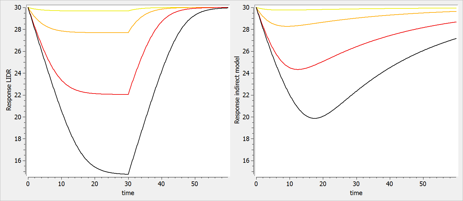
10.mlxEditor
Version 2021
This documentation is for mlxEditor starting from 2021 version.
©Lixoft
mlxEditor is an application to write, edit and organise models written in the mlxtran language. It has mlxtran dedicated features, such as syntax coloring, autocompletion and verification, and is integrated with Monolix and Simulx for easier model development.
 |
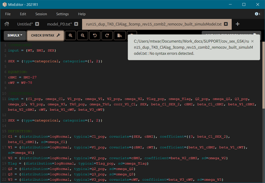 |
Main functions:
- Writing models in the mlxtran language.
- Editing user custom models and models from the Monolix library, which is integrated with the application.
- Editing models directly in the GUI: Monolix (tab: Structural model) and Simulx (Tab: Definition/Model).
- Managing models in work sessions.
Main features:
- Mlxtran syntax coloring for different model elements, such as block definition, parameters, macros.
- Autocompletion for variables, mlxtran keywords, functions (tab-key accepts a selected item).
- Find and Find&Replace.
- Zoom in/out to increase/decrease the font size.
- Syntax check to verify if the mlxtran code is correct and a model can be loaded in Monolix or Simulx.
In the mlxEditor application:
-
- Access to the Monolix libraries,
- Monolix and Simulx syntax check,
- Save and export to Simulx,
- Sessions: collections of models that can be reloaded automatically.
In the GUI edit mode:
-
- Several saving options: Save & apply – saves the model under the same name (overwrites the previous model) and applies it to the current project, Save as & apply – saves the model under a different name and applies it to the current project, Save as – saves the model under a different name without applying to the current project.
- Zoom applied in the edition model remains in the “Tab: Structural model” after closing the edition mode.
11.Share your feedback
Help us improve MlxEditor!
We value your opinion. We would love to hear from you to align our vision and concepts with your needs and expectations. Let’s make sure you get the most of our software.
NB: This is not a support form. Commercial users can contact us via the support email.
12.FAQ
This page summarizes frequent questions about Mlxtran.
In construction