Guidelines to choose a TMDD model

The choice of a model is often not trivial. Because the data may not be sufficient to identify all the parameters of the full model, the parameter estimation process using the full model may not only lead to parameter estimates with large uncertainty but also fail to converge. This page gives guidelines to help the modeler to choose an appropriate TMDD model for his data set. The necessity of using simplified TMDD models is commonly the consequence of a limited data set and should not hide the fact that the reality may be more complex than the model.

In addition to using the TMDD approximation models (which are derived using assumptions on the parameter values), it is also possible to fix the unidentifiable parameter values, for instance using prior knowledge and typical values, while keeping the full TMDD model structure.

When to use a TMDD model How to choose a first model Using prior information Entities measured Shape of the measured concentration Range of doses          Improving the model Bottom-up versus top-down approaches                                                                   Examples of diagnostics

Summary guidelines

When to use a TMDD model

Several aspects can guide the choice of using a TMDD model.
First the type of molecule: biologics such as monoclonal anti-bodies, cytokines, growth factors, fusion proteins, antibody-small molecule drug conjugates or hormones are likely to display TMDD kinetics, at least in a certain concentration range. Notice that even if the biologic is eliminated via a TMDD mechanism, the typical TMDD behavior may not be observable due to too high or too low doses. In this case, a TMDD model will probably be over-parameterized. On the opposite, TMDD models should not be restricted to biologics as small molecules can also display TMDD kinetics (Guohua An (2017) J Clin Pharm 57(2)).

Second, the results of a non-compartmental analysis (NCA) can hint at TMDD kinetics if the apparent volume of distribution or the total clearance vary between the first dose and subsequent doses or for different dose amounts (Levy (1994), Clin Pharm Ther 56(3)).

Third, the shapes of the concentration-time curves is a key aspect. It will help to detect a TMDD behavior but also to choose the appropriate TMDD model among the several approximations possible.

How to choose a first model

Using prior information

The order of magnitude for some parameters might have been measured directly, for instance with in vitro experiments (e.g Biacore experiments, which usually provide kon and koff). This information can be used to choose an appropriate approximation:

• evidence of fast binding to receptor (high kon and koff) => QE, Wagner, MM
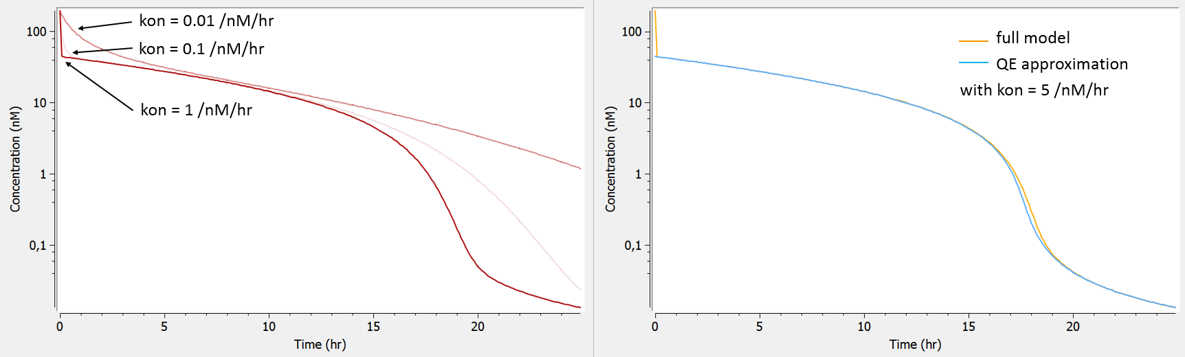
  The influence of the kon parameter on the concentration-time curve is depicted below using Mlxplore, for typical parameter values. When kon is large, the initial drop of concentration due to the binding of the drug to the target is so fast that no data has been recorded in this part of the curve, therefore preventing a reliable estimation of kon. In this case, as can be seen on the right, the QE approximation gives the same concentration-time curve as the full model, except for the initial drop (phase 1).
  test
• evidence of irreversible binding to receptor (very low dissociation constant KD) => IB, “const. Rtot + IB”, MM
  The dissociation constant KD controls the height of the last phase (phase 4). When the binding affinity is very strong and thus the KD low, the last phase of the concentration-time curve is often below the LOQ and cannot be measured. In that case it is not possible to estimate KD and one can assume that the binding is irreversible. As can be seen on the left panel, the full model and the IB approximation model will differ in a part of the curve in which anyway no data had been recorded.
  test
• evidence of similar rates for the elimination of free and bound receptor (kdeg and kint) => constant Rtot, Wagner, “const. Rtot + IB”, MM
  In the plot below (left), we show the total concentration of receptor. When kint is larger than kdeg, the total receptor concentration will decrease after the ligand administration. Indeed, part of the receptor is then bound to the ligand and the complex is eliminated faster than the free receptor (kint>kdeg). Is is often the case in practice, as the binding of the ligand promotes the internalization of the receptor. On the opposite, when kint<kdeg, the total receptor concentration increases. Finally, when the complex internalization rate kint and the receptor degradation rate kdeg are very similar, the total receptor concentration is constant. The equation for the total receptor can then be dropped leading to a system with less parameters to estimate. When truly kint=kdeg, the constant Rtot model perfectly superimpose with the full model (right panel).
   test

Entities measured

Usually, in the case of a soluble target, the total ligand concentration (Ltot) is available, and sometimes the free ligand concentration (L) and/or the total target concentration (Rtot). For membrane-bound targets, usually the free ligand concentration (L) is available, and sometimes the target occupancy (TO) (see Gibiansky et al. PAGE 2011 Talk).
The following outputs are available for all models except the MM model: free ligand L, total ligand Ltot, free receptor R, total receptor Rtot, complex P, target occupancy TO and ratio of free receptor to baseline RR. Here are the restrictions in the model choice depending on the measured entities:

• only free ligand L measured => all models
• any other combination of measured entities => all models except MM

Shape of measured concentrations

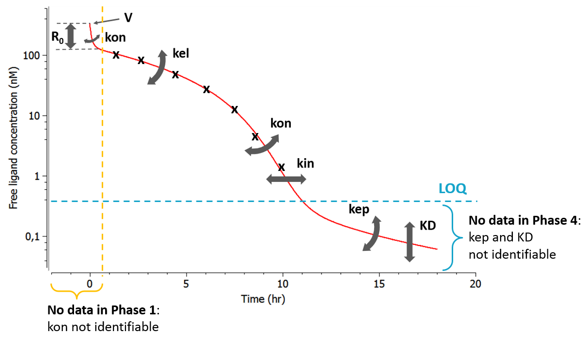
As can be seen in the overview figure, the different approximations lead to different typical concentration shapes. As a consequence, the shape of the measured concentrations is a key element to choose an appropriate model. Two situations are particularly common: first, if the binding of the drug to the target is fast, phase 1 will be very short (in time) and measurements may only start after phase 1. In this case, the parameters related to the binding (especially kon) will not be identifiable and one can assume rapid-binding. Second, it may be that phase 4 appears at very low concentrations that are below the limit of quantification (LOQ). This may happen if the dissociation constant KD is small, i.e if the binding is almost irreversible.

• phase 1 not observable due to too rapid binding => QE, Wagner, MM
• phase 4 not observable because below LOQ => IB, “const. Rtot + IB”, MM

Range of doses

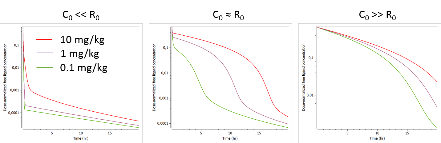
The initial receptor concentration R0 and the volume of the central compartment V have a similar influence on the ligand concentration-time curve, except that the shift induced by a volume change is dose-independent (same shift for all doses), while that induced by a change in R0 is dose-dependent (larger shift for small doses). If the tested doses do not range over a sufficient range, R0 may be difficult to identify. In this case the MM model may be a good approximation. If the MM model is not possible or insufficient, it is also possible to fix the value of R0.

The plots below show the concentration-time profile for different initial receptor concentrations (related to the receptor production and degradation rates via ).

• C0>>R0: When the initial drug concentration (calculated as Dose/V) is small compared to the initial reception concentration, we recover the low dose case presented above, where only phase 1 and phase 4 can be seen.
• C0≈R0: When the initial ligand and receptor concentrations are of the same order of magnitude, the typical TMDD concentration-time curve shape is observed. The initial drop appears clearly and is dose-dependent. If several doses are tested, R0 (i.e kdeg) is likely to be identifiable.
• C0<<R0: When the initial drug concentration is much larger than the initial receptor concentration (which is often the case), the initial drop due to binding to the receptor is small on the scale of the ligand concentration and probably hard to quantify in the presence of measurement noise. In this case, the parameter R0 (or kdeg using the usual parameterization) which influences the height of the initial drop is usually not identifiable.

Improving the model

Bottom-up versus top-down approaches

A top-down approach to find an appropriate TMDD model has been proposed in Gibiansky et al. (2008), JPP 35(5). The procedure is the following: (i) fit the data with the full TMDD model, (ii) use the estimated parameters to simulate typical concentration-time curves with the full model and the approximations, (iii) if the simulations using a approximation are equivalent to the simulations with the full model, the approximation should be used. The strong disadvantage of this method is that the fitting of the full model may not converge, or give very uncertain estimates that are not informative and not reliable for simulations.

On the opposite, in a bottom-up approach, simpler models are tested first and progressively complexified if mis-specifications are detected in the diagnostic plots. Depending on the prior information, the first tested model can be any typical PK or TMDD model, and the diagnostic plots can help improving the model by removing one or several assumptions, in one or several steps. We recommend to use the bottom-up approach.

test

Examples of diagnostics

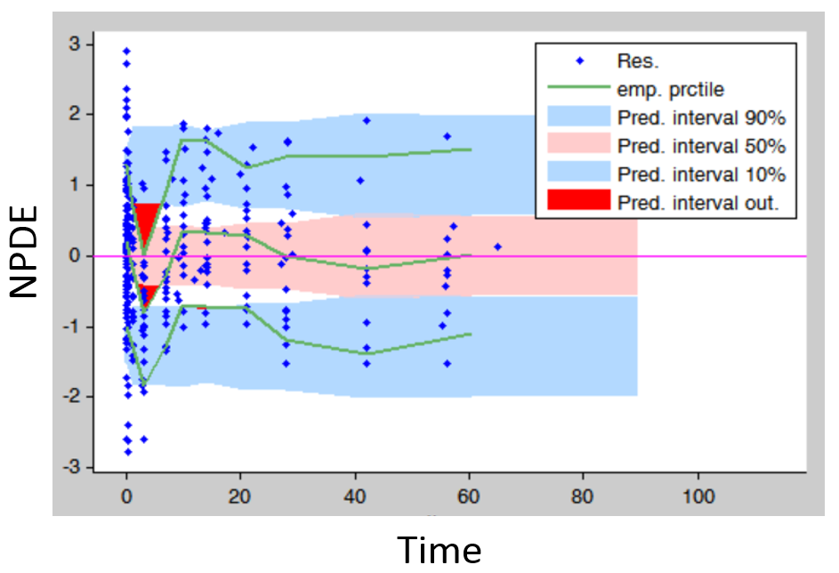
• Residuals (population weighted residuals, individual weighted residuals or normalized prediction distribution errors versus time or predictions): residuals plots help to detect if the model performs poorly for some specific times ranges or concentration ranges. Stratifying by dose group also permits to detect dose-dependent trends. An example is given below. The trend in the residuals indicates a model mis-specification. In this case a more complex model (with more parameters and thus more flexibility) can be tried. 

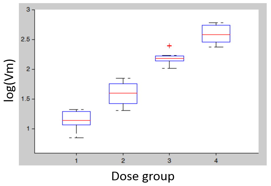
• Covariates: plotting the distribution of parameter values (or of random effects) for the different dose groups (which needs to be considered as a categorical covariate) allows to detect dose-dependent trends that indicate a model mis-specification. In the figure below (left), the individual parameters distribution of Vm is stratified by dose and shows a significant trend with increasing doses. This indicates that a more complex model is needed.
  
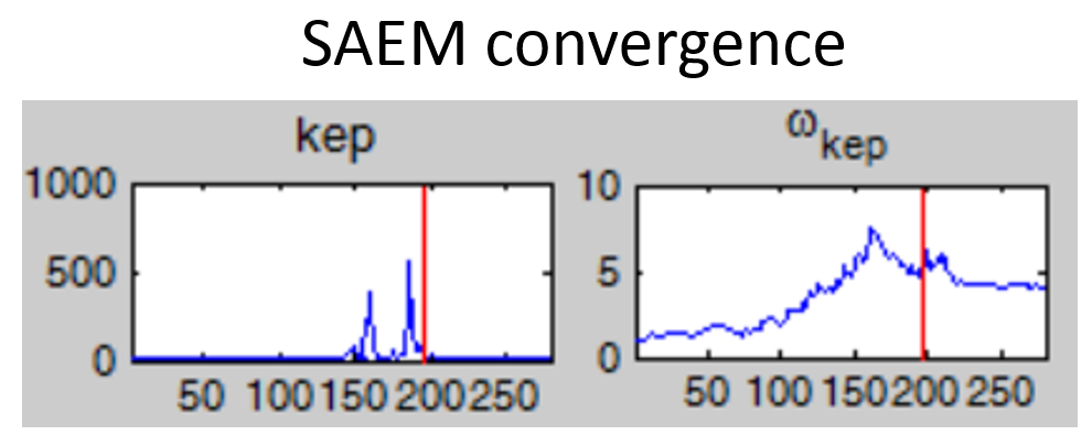
• Non-convergence of SAEM: if the fixed effect estimates is unstable and/or the omega value representing the standard deviation of the random effects converges to a very high value (see example below), the model is probably over-parameterized. Several options are possible to reduce the model complexity: (i) remove the inter-individual variability on this parameter, (ii) fix the value of the parameter, (iii) choose a model with less parameters.
  
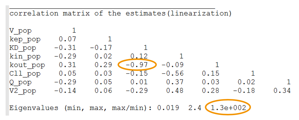
• High condition number: the condition number is the ratio of  the largest eigenvalue of the correlation matrix over the smallest value. High condition numbers hint at high correlations between parameters and thus model over-parameterizations. As a rule of thumb, condition numbers below 10 are ok, between 10 and 100 the model can be questionable, and above 100 the model is likely to be over-parameterized. In the example below, the high condition number probably reflects the high correlation between kdeg (kout) and KD. When the Monolix project is exported to Mlxplore using the last estimated parameters, one indeed clearly see that the influence of kdeg and KD on the concentration-time curve is the same. It will therefore not be possible to identify both.  In this case, options are: (i) fix the value of one of the two parameters, or (ii) choose a model with less parameters.
  test
• High r.s.e values: the r.s.e values indicate how uncertain the parameter estimate is. A high uncertainty may be the result of the parameter being unidentifiable because of lacking data. If a fixed parameter has a high r.s.e, one can try to either remove the IIV on this parameter, or fix this parameter value or try a model with less parameters. When an omega has a high r.s.e, one can try to remove the IIV on this parameter.
  

Conclusion

1. Visualize and explore the data before starting the modeling.
2. Have in mind how the parameters influence the curves. It is possible to check the influence for specific parameter sets with Mlxplore.
3. Use the graphics to diagnose the model.
4. Try several models, the librairie makes it easy.
5. Consider several levels of flexibility:
   • different model approximations, and 1 or 2 compartments
   • parameters estimated or fixed
   • parameters with or without inter-individual variability
6. Keep in mind the ultimate modeling goal.