A wide range of ODEs models for tumour growth (TG) and tumour growth inhibition (TGI) is available in the literature and correspond to different hypotheses on the tumor or treatment dynamics. In the absence of detailed biological knowledge, selecting the most appropriate model is a challenge. In MonolixSuite2020, we provide a modular TG/TGI model library that combines sets of frequently used basic models and possible additional features. This library permits to easily test and combine different hypotheses for the tumor growth kinetics and effect of a treatment, allowing to fit a large variety of tumor size data.
When available, analytical solutions are used.
Tumor growth models
Initial tumor size
The initial tumour size TS0 can be either be:
- a parameter to estimate,
- a regressor to read from the dataset.
It has to be noted that the time corresponding to the initial tumour size is not necessarily 0. It is the case for models implemented with an analytical solution, but for models implemented with an ODE system it corresponds to the initial integration time. This time is not fixed for most models from this library, which means that it is by default the first dose or observation time in the data set, and can vary between individuals. If one wishes to fix the initial integration time for all individuals, one can uncomment the line “t_0=0” in the model to fix the initial integration time at 0, and modify the line to choose another initial time, which must necessarily be before any dose or observation in the data set. Thus only models implemented with an analytical solution can capture observations at prior times than the time for TS0.
Kinetics of tumor growth
After a growing phase, tumors experience a saturation due to limits of nutrient supply. However, this saturation property is often never measured in patients in practice because the host dies in the majority of cases before this saturation phase begins. Also in preclinics, the experiments have to be canceled if a specific tumor size is reached due to ethical reasons. Thus, tumor growth models may be divided into two broad categories: those which are able to capture the saturation as the tumor grows (achieved by the introduction a carrying capacity or a spontaneous decay component) and those which do not.

-
Models without saturation
-
Linear
-
The linear tumor growth assumes a constant zero-order growth rate.
| ODE system | Analytical solution | 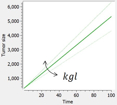 |
|
$$ \frac{dTS}{dt} = kgl $$ $$ TS(t_0)=TS0 $$ |
$$ TS=kgl*t+TS0 $$ |
-
-
Quadratic
-
The quadratric tumor growth combines linear and quadratic growth rates. Because time is involved in this model, the initial time is fixed to 0 in corresponding library models.
| ODE system | Analytical solution | 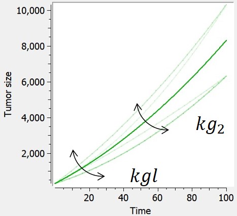 |
|
$$ \frac{dTS}{dt} = kgl+2*kg2*t $$ $$ TS(t_0)=TS0 $$ |
$$ TS=kgl*t+kg2*t^2+TS0 $$ |
-
-
Exponential
-
The exponential growth assumes the growth rate of a tumor is proportional to tumor burden (first-order growth).
| ODE system | Analytical solution |  |
|
$$ \frac{dTS}{dt} = kge*TS $$ $$ TS(t_0)=TS0 $$ undefined |
$$ TS=TS0*e^{kge*t} $$ |
-
-
Power law
-
If 0 < gamma < 1, the power law model (also named generalized exponential) provides a description in terms of a geometrical feature of the proliferative tissue: the growth rate is proportional to the number of proliferative cells as a fraction of the full tumor volume. The case gamma=1 corresponds to proliferative cells uniformly distributed within the tumor and leads to exponential growth. The case gamma=2/3 represents a proliferative rim limited to the surface of the tumor, where the tumor radius grows linearly in time.
| ODE system | Analytical solution | 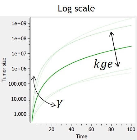 |
|
$$ \frac{dTS}{dt} = kge*TS^\gamma $$ $$ TS(t_0)=TS0 $$ |
$$ TS=(kge*(1-\gamma)*t+TS0^{1-\gamma})^{\frac{1}{1-\gamma}} $$ |
-
-
Exponential-linear
-
Experimental data of tumor growth in untreated xenograft mice suggest that tumor growth dynamics follow two distinctively different phases of growth: an initial exponential growth, followed by a linear growth phase. Biologically, this is due to the fact that the growth of the tumor is almost unlimited at first, but that as the nutrients go scarce, its growth is then necessarily restricted.
The simple exponential-linear model captures this with a transition between an exponential (first-order) growth to a linear (zero-order) growth. The transition time is computed to ensure that the solution is continuously differentiable, but this is possible only if the model is not combined with any treatment effect or additional features. In that case, the transition time corresponds to TS = kgl/kge.
In the library, the exponential-linear model is provided with its analytical solution and can not be combined to any treatment effect or additional features.
| ODE system | Analytical solution | 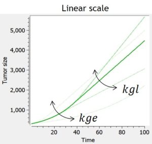 |
|
$$ \frac{dTS}{dt} = kge*TS, t\le\tau$$ $$ \frac{dTS}{dt} = kgl, t\ge\tau$$ $$ TS(t_0)=TS0 $$ $$\tau = \frac{1}{kge}ln(\frac{kgl}{kg*TS0})$$ |
$$ TS=TS0*e^{kge*t}, t\le\tau $$
$$ TS=kgl*(t-\tau)+TS0*e^{kge*\tau}, t\ge\tau $$ $$\tau = \frac{1}{kge}ln(\frac{kgl}{kg*TS0})$$ |
-
-
Simeoni
-
The Simeoni model approximates the exponential-linear model with a single differential equation. The power term is fixed to 20 to allow the system to pass from the first-order to the zero-order growth sharply enough, as in the original system. With this value, the growth rate is approximated by kge*TS when TS is smaller than kgl/kge, and by kgl when TS is larger than kgl/kge. The advantage of the Simeoni model over the exponential-linear model is that it is differentiable even when combined with any type of treatment effect.
When used in combination with the description of non-proliferating subpopulations of cells (transit compartments with cell distribution, or two populations model), with TS the size of the proliferating subpopulation, the growth function is slowed down by the factor TS/TotalTS only when the tumor is in its linear growth phase, but not in the exponential growth phase.
| ODE system | Reference | 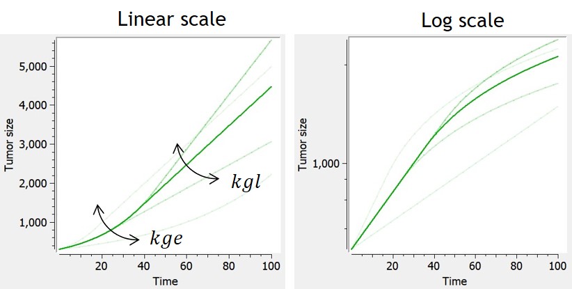 |
|
$$ \frac{dTS}{dt} = \frac{kge*TS}{(1+(\frac{kge}{kgl}*TS)^\psi)^(\frac{1}{\psi}} $$ $$ TS(t_0)=TS0 $$ |
Simeoni et al. (2004). |
-
-
Koch
-
Similarly to the exponential-linear and Simeoni models, the Koch tumor growth model is a nonlinear growth function that follows an initial exponential growth followed by a linear growth phase. Its particularity is a smooth transition between exponential and linear growth phase, rather than a rapid switch after a threshold reached for the time (exponential-linear) or tumor size (Simeoni).
When used in combination with the description of non-proliferating subpopulations of cells (transit compartments with cell distribution, or two populations model), with TS the size of the proliferating subpopulation, the growth function is slowed down by the factor TS/TotalTS.
| ODE system | Analytical solution | Reference | 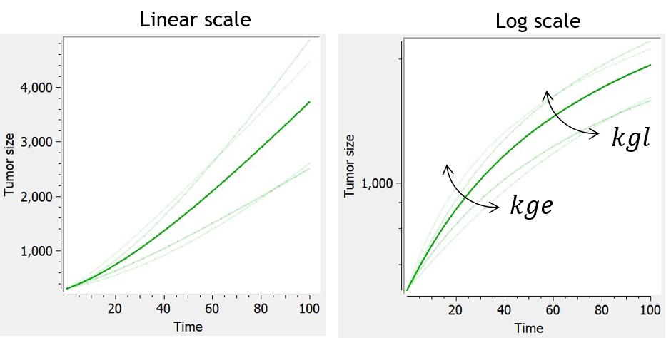 |
|
$$ \frac{dTS}{dt} = \frac{2kge*kgl*TS}{kgl+2kge*TS} $$ $$ TS(t_0)=TS0 $$ |
$$ TS=TS0e^{2kge(t+\frac{1}{kgl}(TS0-TS))} $$ | Koch et al. (2009) |
-
Models with saturation
-
Logistic
-
This model assumes an exponential growth rate which decelerates linearly with respect to the tumor size. This results in sigmoidal dynamics – with an initial exponential growth phase followed by a growth-saturated phase as the tumor reaches its carrying capacity (TSmax).
| ODE system | Analytical solution | 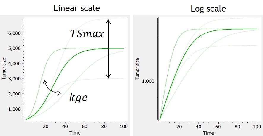 |
|
$$ \frac{dTS}{dt} = kge*TS(1-\frac{TS}{TSmax}) $$ $$ TS(t_0)=TS0 $$ |
$$ TS=\frac{TSmax*TS0}{TS0+(TSmax-TS0)*e^{-kge*t}} $$ |
-
-
Generalized logistic
-
In this model, tumor growth depends on tumor size with a generalized logistic function. It reduces to the logistic model if 

| ODE system | Analytical solution | 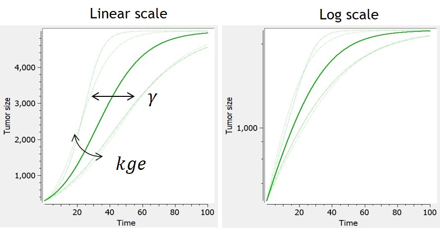 |
|
$$ \frac{dTS}{dt} = kge*TS(1-(\frac{TS}{TSmax})^{\gamma}) $$ $$ TS(t_0)=TS0 $$ |
$$ TS=\frac{TSmax*TS0}{(TS0^\gamma+(TSmax^\gamma-TS0^\gamma)*e^{-kge*\gamma*t})^{\frac{1}{\gamma}}} $$ |
-
-
Simeoni-logistic
-
In [Haddish-Berhane et al., 2013], a hybrid model derived from the Simeoni model is proposed, that combines exponential, linear and logistic growth.
| ODE system | Reference | 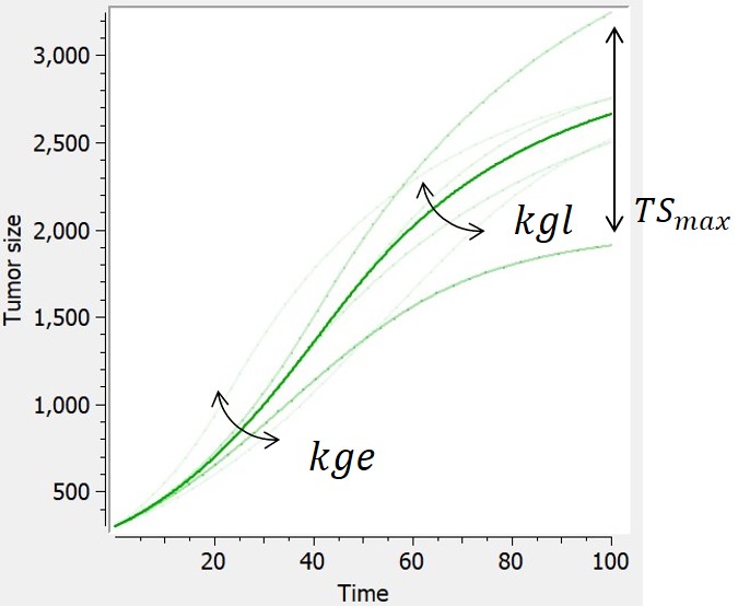 |
|
$$ \frac{dTS}{dt} = \frac{kge*TS*(1-\frac{TS}{TSmax})}{(1+(\frac{kge}{kgl}*TS)^\psi)^{\frac{1}{\psi}}} $$ $$ TS(t_0)=TS0 $$ |
Haddish-Berhane et al., 2013 |
-
-
Gompertz
-
The Gompertz model follows the observation of a deceleration of the growth rate over time, without any phase at which the growth rate remains constant. The volume converges asymptotically to ")
Several parameterizations can be used, and two are displayed on the table below. The first parameterization is the one implemented in the library, and the one for which the impacts of the parameters are the most separate and easiest to control. However, the carrying capacity TSmax can be difficult to estimate and can lack biological meaning if no clear tumor size saturation is seen. With the second parameterization, alpha and beta have an impact on the carrying capacity and on the growth rate, while TS0 also has an impact on the carrying capacity.
| ODE system | Analytical solution | |
|
$$ \frac{dTS}{dt} = TS*\beta*ln(\frac{TSmax}{TS}) $$ $$ TS(t_0)=TS0 $$ |
$$ TS=TSmax*e^{e^{-\beta*t}*ln(\frac{TS0}{TSmax})} $$ | 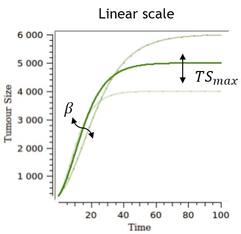 |
| $$ \frac{dTS}{dt} = \alpha*e^{-\beta*t}*TS $$
or, equivalently, $$ \frac{dTS}{dt} = (\alpha-\beta*ln(TS))TS $$ $$ TS(t_0)=TS0 $$ |
$$ TS=TSmax*e^{e^{-\beta*t}*ln(\frac{TS0}{TSmax})} $$ | 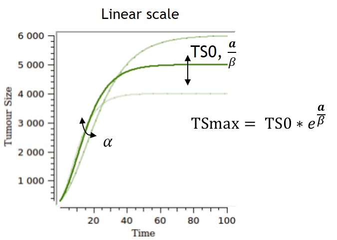 |
-
-
Exponential-Gompertz
-
An exponential-Gompertz model can also be considered, built upon the assumption that the tumor follows at first an exponential growth, and is then akin to a Gompertz model once the nutrients start to go scarce.
| ODE system | Refefence | 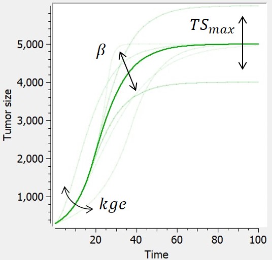 |
|
$$ \frac{dTS}{dt} = min(kge*TS,TS*\beta*ln(\frac{TSmax}{TS})) $$ $$ TS(t_0)=TS0 $$ |
Wheldon (1988) |
-
-
Von Bertalanffy
-
This model is based on balance equations of metabolic processes. The growth is limited with a loss term.
| ODE system | Analytical solution | Reference | 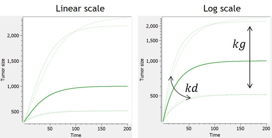 |
|
$$ \frac{dTS}{dt} = kg*TS^{2/3}-kd*TS $$ $$ TS(t_0)=TS0 $$ |
$$ TS= \left[ \frac{kg}{kd}+(TS0^{1/3}-\frac{kg}{kd})*e^{-1/3*kd*t} \right]^3 $$ | Von Bertalanffy, 1957 |
-
-
Generalized Von Bertalanffy
-
This is the generalized version of the Von Bertalanffy model. The von Bertalanffy model corresponds to the case gamma=⅔, where the growth is proportional to the surface of the tumor.
The loss term induces for some parameter values a saturation of the tumor, with ^{\frac{1}{1-\gamma}}")
When the Von Bertalanffy model (or generalized Von Bertalanffy model) is used in combination with a tumor inhibition model which makes use of the Norton Simon killing hypothesis, the treatment effect is only applied to the growth term of the model (and not to its decay term).
| ODE system | Analytical solution | Reference | 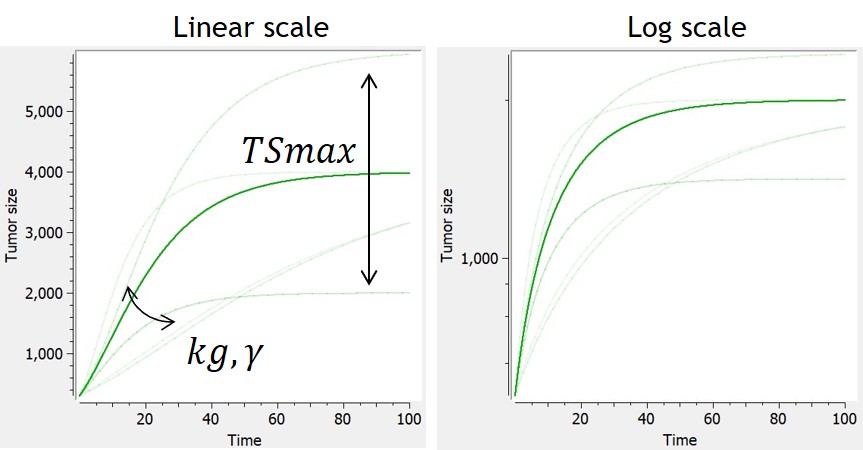 |
|
$$ \frac{dTS}{dt} = kg*TS^{\gamma}-kd*TS $$ $$ 0 \leq \gamma \leq 1 $$ $$ TS(t_0)=TS0 $$ |
$$ TS= \left[ \frac{kg}{kd}+(TS0^{1-\gamma}-\frac{kg}{kd})*e^{-(1-\gamma)*kd*t} \right]^\frac{1}{1-\gamma} $$ | Von Bertalanffy, 1957 |
Additional features
Additional features can be included to consider more complex tumor growth models:
-
Dynamic carrying capacity due to angiogenesis
The library includes, as an example, a module taken from Hahnfeldt et al,1999 that models the effect of angiogenesis as a dynamic carrying-capacity. When selecting the dynamic carrying-capacity module, TSmax is defined as an ODE variable instead of a constant parameter, with the following ODE:
| ODE | Reference | 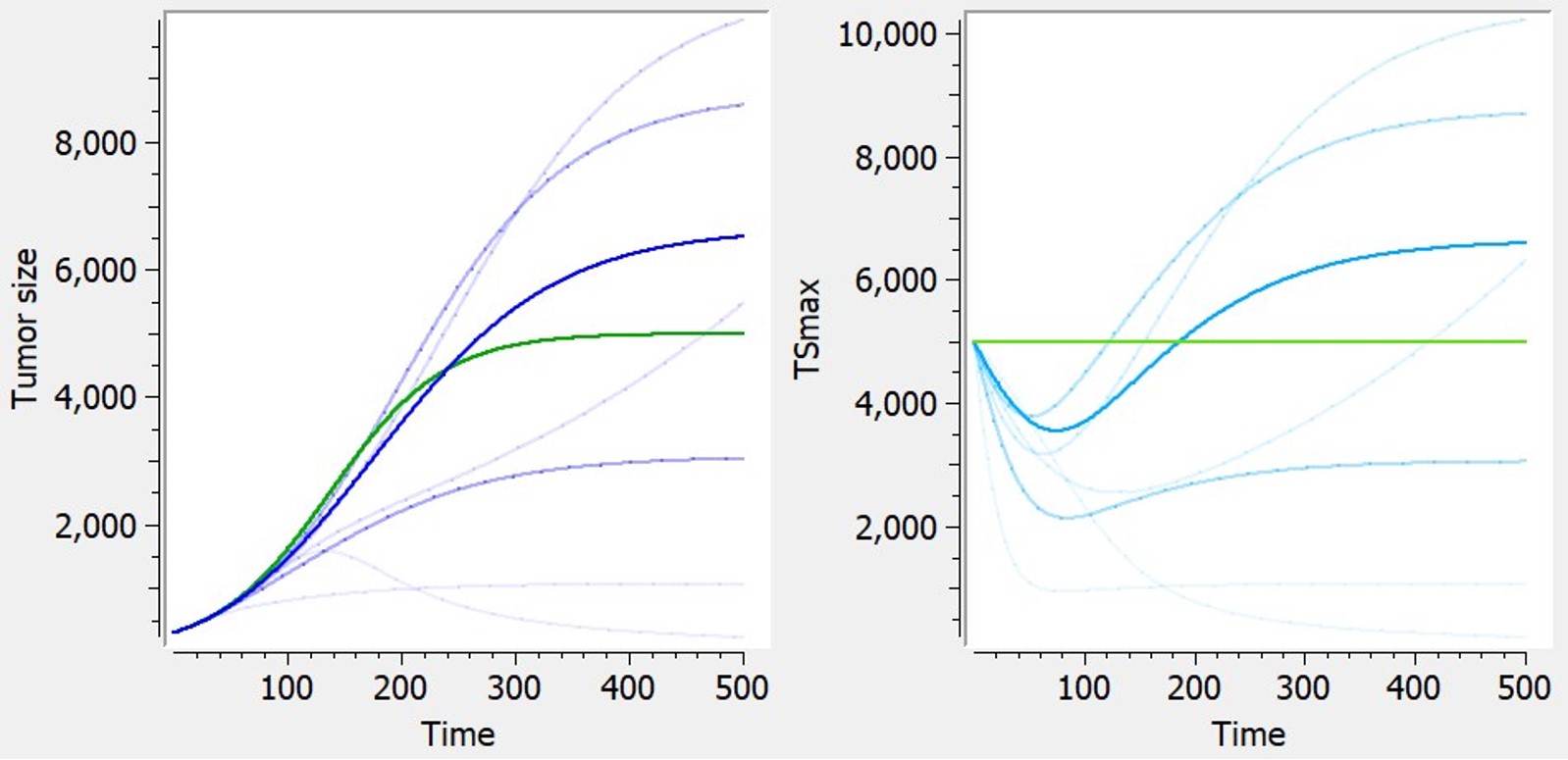 Examples of curves for tumor size (left) or carrying capacity (right) with diverse shapes, based on logistic tumor growth. Green: predictions without the additional feature (constant TSmax). Blue: with dynamic carrying capacity. Examples of curves for tumor size (left) or carrying capacity (right) with diverse shapes, based on logistic tumor growth. Green: predictions without the additional feature (constant TSmax). Blue: with dynamic carrying capacity. |
|
$$ \frac{dTS_{max}}{dt} = kp_v*TS -\kappa*TS_{max} – kd_{\nu}*TS*TS^{2/3} $$ |
Hahnfeldt et al,1999 |
-
Immune dynamics causing shrinkage or oscillations of tumor size
The library includes, as an example, a model of tumor-immune interactions with chemotherapy proposed by De Pillis et al. (2007), taking into account the control of the tumor growth by the immune system, and the weakening of the immune system as a side effect of chemotherapy. The model includes an additional ODE defining effector–immune cells:
| ODE system | Reference | 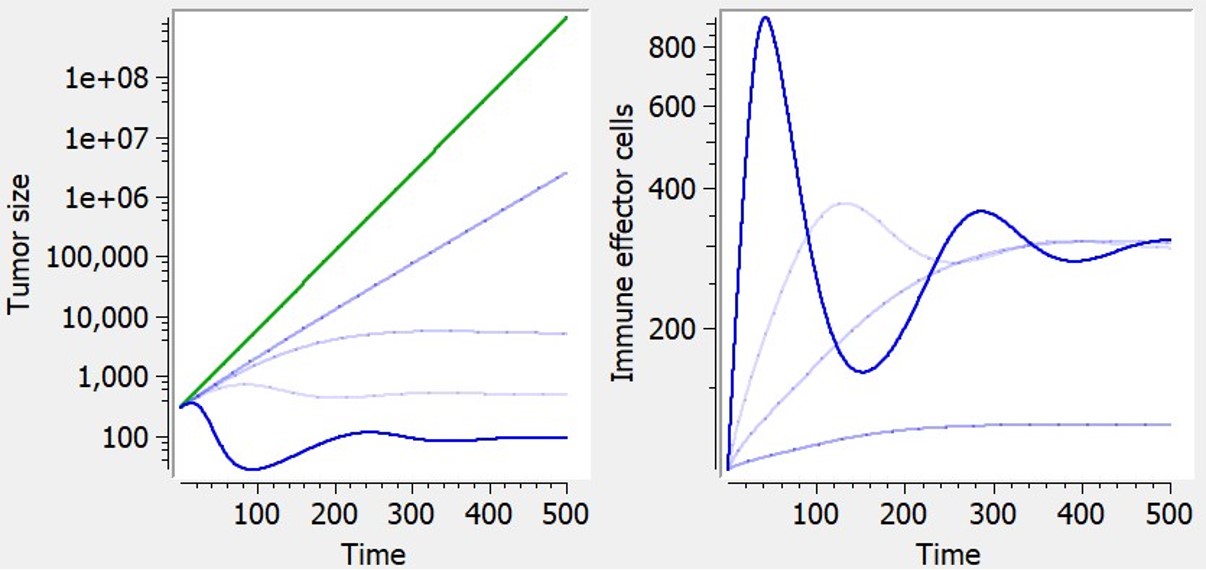 Examples of curves for tumor size (left) or effector immune cells (right) with diverse shapes, based on exponential tumor growth. Green: prediction without the additional feature (constant tumor growth). Blue: with immune dynamics. Examples of curves for tumor size (left) or effector immune cells (right) with diverse shapes, based on exponential tumor growth. Green: prediction without the additional feature (constant tumor growth). Blue: with immune dynamics. |
|
$$ \frac{dTS}{dt} = growth -ki*I*TS $$ |
De Pillis et al. (2007) |
More details on these additional features.
Treatment effect
Type of treatment
Flexible treatment definition is provided thanks to several possibilities:
- No treatment
This option corresponds to simple tumor growth models.
- PK model
Dosing information is encoded in the dataset, and the effect of the treatment is modeled via a simple PK model (one compartment, bolus administration, linear elimination) which can be easily adapted to a more complex model or to fix some parameters. The predicted concentration inhibits tumor size.
Note that in case of a high number of doses, it is preferable to approximate the exposure by a piecewise regressor or by a constant treatment, to reduce computation cost. Particularly when the dosing is daily and the disease lasts several years, modeling of the PK is not useful and very costly.
- Exposure as regressor
Values which describe the evolution of the treatment’s exposure/concentration with respect to time are already stored within the data set and are used within the TGI model under the variable EXPOSURE.
DATA FORMAT RESTRICTIONS: The values describing the treatment’s exposure with respect to time must be stored in a separate column of the data set labelled ‘REGRESSOR’.
- Treatment start at t=0
The tumour growth inhibition component is applied with a constant effect after t=0.
DATA FORMAT RESTRICTIONS: The data must be formatted as to have the treatment being added at time t=0 for all individuals. Measurements before that can make use of negative values for time. Note that in that case, the initial integration time (corresponding to the initial tumour size TS0) is the first measurement time and can vary between individuals.
- Treatment start time as regressor
The time at which the treatment is added is a variable named T in the model, which may vary between individual, and whose value is read from a regressor column in the data set. When time t<T, a simple tumour growth model is being implemented. After, a tumour growth inhibition component to the model is added.
DATA FORMAT RESTRICTIONS: The values for T must be stored within the data set in a separate column tagged as ‘REGRESSOR’.
- No treatment (0) vs treatment (1) regressor
A simple tumour growth model is being implemented if the variable Trt = 0. If Trt = 1, a tumour growth inhibition component to the model is added. Trt is read from a regressor column in the dataset.
DATA FORMAT RESTRICTIONS: A 0 – if the measurement was taken before or after treatment – or 1 – if it was taken during treatment – must be matched and stored within a separate column under the header ‘REGRESSOR’ for each of the measurements of the data set.
Killing hypothesis
There are two different most commonly used hypothesis relevant to the method of killing of any given treatment within the literature:
|
|
If the growth is exponential (
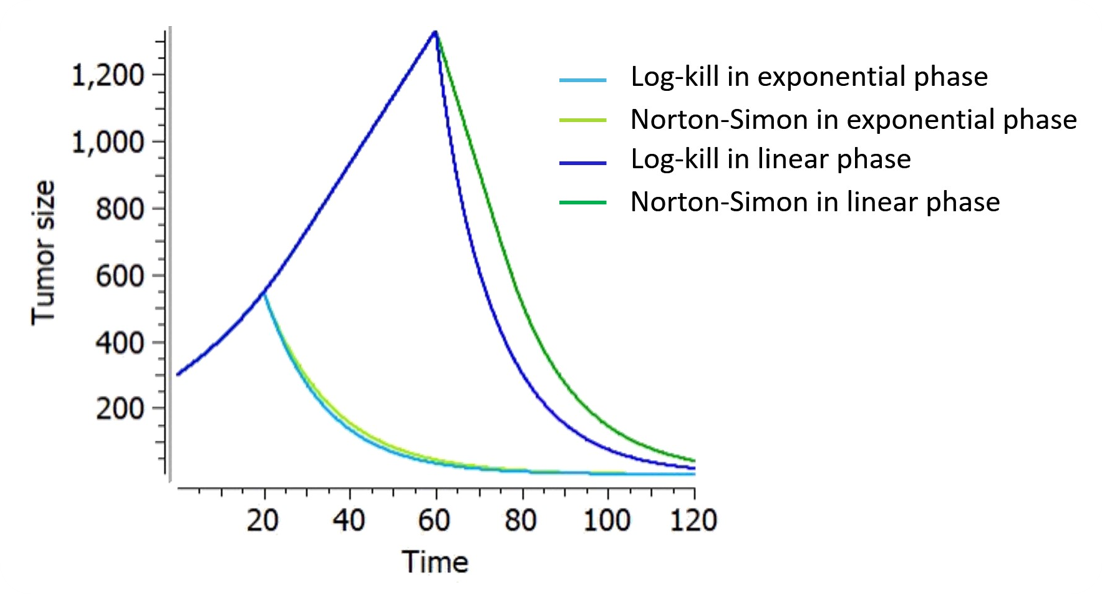
On the figure on the right for example, the tumor size follows an exponential-linear growth, a constant treatment effect is applied either in the exponential phase (at t=20) or in the linear phase (at t=60). The treatment kinetics is linear. The parameters are adapted such that 
It enfolds that under the Norton-Simon hypothesis the optimal treatment should deliver the most effective dose level of drug over as short a time as possible (high dose density), since tumors given less time to grow between treatments are more likely to be eradicated.
Dynamics of treatment effect
Five different exposure-dependent treatment kinetics which we found to be most common within the literature can be combined with both of these killing hypotheses.
Below are plots showing the curves resulting from the addition of these TGI models to an exponential TG model, with a punctual drug exposure resulting from a single dose which is absorbed at time 0 and then eliminated. On the first figure, a linear range of different dose amounts has been applied in order to exhibit the linear and non-linear relationships between exposure and treatment effect.

When the treatment exposure is not given, the treatment effect is constant.
Delay of treatment effect
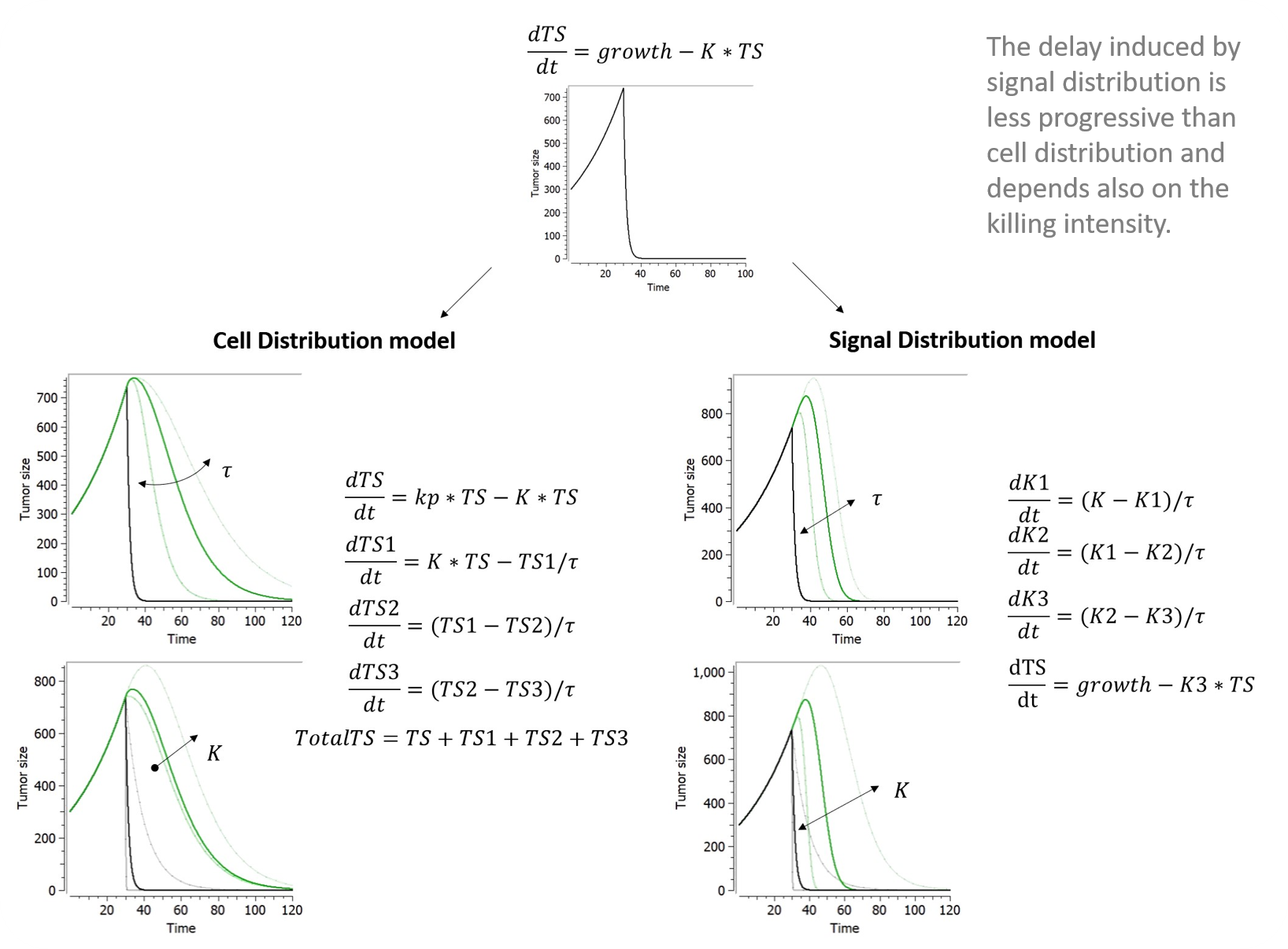
Chemotherapeutic effects often appear days or weeks following drug exposure. To account for a more progressive tumour regression, a delay in either the treatment effect (i.e. signal distribution model) or cell death (i.e. cell distribution model) may be added via transit compartments.
-
Signal distribution model
Lobo and Balthasar (2002) applied to tumor growth the transit compartment model proposed by Sun & Jusko (1998) to characterize delayed drug effects that occur via a cascade or signal transduction. The operative rate function of tumor cells killing, K3, is related to K via a series of transit compartments (K1-K3). Tau refers to the mean transit time in each transit compartment. Although 4 transit compartments were used in Lobo and Balthasar (2002), the model implemented in our library has only 3 compartments for an easier comparison to the cell distribution model. It can be easily edited by the user to add more compartments if nedded.
-
Cell distribution model
The cell distribution model proposed in Simeoni et al., 2004 assumes that the anticancer treatment makes some cells non-proliferating. These cells pass through different stages (also called transit compartments), characterized by progressive degrees of damage, and, eventually, they die. Hence, the attacked tumor cells have a lifespan.
The number of stages of damage and the value of tau affect the shape of the distribution of the time-to-death of damaged tumor cells. The lifespan, or time-to-death, of the attacked tumor cells, is the mean transit time that it takes for the tumor cells, affected by the action of a drug, to go through the cascade of damaging events to cell death. For n transit compartments, the average lifespan is computed by Mtt = n*tau. This library includes an implementation of the model with three transit compartments, as in Simeoni et al., 2004.
When the model considers two populations of cancer cells in the tumor (sensitive/resistant), the treatment induces the transfer or both types of cells into the first transit compartment, with different rates.
Below are plots showing the curves resulting from the addition of both of these delays to a model making use of exponential TG component and a log-kill constant TGI component depending on constant treatment starting at time 30.
Emergence of resistance
A common feature of tumours is the emergence of treatment-resistance. This phenomena can be modelled in a variety of ways. Decrease in treatment efficacy can be simply added in a phenomenological approach. More mechanistic models try to represent the cell population in its heterogeneity, splitting it into at least two subpopulations: the proliferating and the quiescent cells.
In this library, we included two common methods used within the literature to achieve this:
-
Claret exponential
This simple phenomenological model accounts for the loss of drug-induced decay over time due to declining efficacy of the drug, which can be due to the emergence of resistance. It uses a single resistance parameter 
| Equation | Refefence | 
Figure for an exponential growth function and constant treatment effect starting at time t=0. |
|
$$ K’ = K*e^{-\lambda*t} $$ |
Claret et al. (2009) |
-
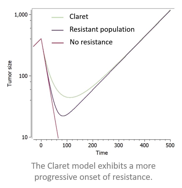
Resistant population
There are many models in the literature that apply variations of the same approach based on two tumor cell populations with different sensitivities, for example Hahnfeldt et al., 2003, Desmée et al., 2017, Lobo & Balthasar, 2002, Jusko, (1973). We have integrated in the library simple versions inspired by this principle, combined with different treatment effects: these models assumes that a fraction of the tumor is resistant to the treatment, thus being killed with a smaller rate than the sensitive part of the tumor. They use a parameter f as initial fraction of resistant tumour cells, and the number of parameters characterizing the treatment effect doubles to have population-specific effects.
| Equation | 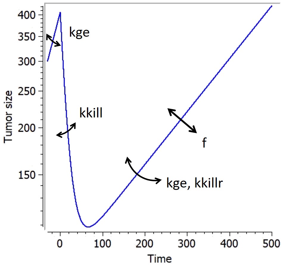
Figure for an exponential growth function and constant treatment effect starting at time t=0. |
| Log-killl hypothesis:
$$ \frac{dTS_s}{dt} = growth – TS_s*K_{TS_s}$$ $$ \frac{dTS_r}{dt} = growth – TS_r*K_{TS_r}$$ Norton-Simon hypothesis: $$ \frac{dTS_s}{dt} = growth * (1- K_{TS_s})$$ $$ \frac{dTS_r}{dt} = growth *(1-K_{TS_r})$$ Initial conditions: $$ TS_s(t_0)=TS0*(1-f) $$ $$ TS_r(t_0)=TS0*f $$ |
Below is a figure showing the curves resulting from the addition of these two resistance components to a model making use of exponential TG component and a log-kill linear TGI component, with a constant treatment effect starting at time 0.
Effect of treatment on angiogenesis or immune dynamics
If more complexity was added to the TG model by means of modelling immune dynamics or a dynamic carrying capacity, it can be decided that these should also be influenced by the addition of a treatment.
-
Combination therapy with active inhibition of angiogenesis
Combination therapy is often used to maximise chances of tumour regression and minimise chances of treatment-resistant clones from emerging. As such, it may be wished to model the effect of an angiogenesis inhibitor, on top of the tumour inhibitor. This corresponds to an additional option named “Additional treatment effect” available in the library when both angiogenesis and a treatment effect are selected. In that case the ODE for TSmax becomes:
$$ \frac{dTS_{max}}{dt} = kp_v*TS -\kappa*TS_{max} – kd_{\nu}*TS*TS^{2/3} -e*TS_{max} $$
The treatment on angiogenesis is added as a second constant treatment (on top of the one selected earlier on). By choosing this additional option, it is assumed that no PK data is available for this second treatment and consequently, first-order kinetics are used to model the effect. Furthermore, the effect of the second treatment is assumed to follow a log-cell kill killing hypothesis.
-
Combination therapy with decay of immune cells
If the treatment added does not only target tumour cells but a more general cell population (such as chemotherapy), it may be relevant to include a killing term on the immune cell dynamics as well. This feature is available in the library if modelling of immune dynamics was selected during selection of tumour growth model. It consists in adding an extra decay constant to take into consideration the effect chemotherapy will have on immune cells. The equations then become:
$$ \frac{dI}{dt} = kp_i – kd_i*I + g*\frac{TS}{h+TS}*I -p*I*TS – K_i*I $$
where the killing term 
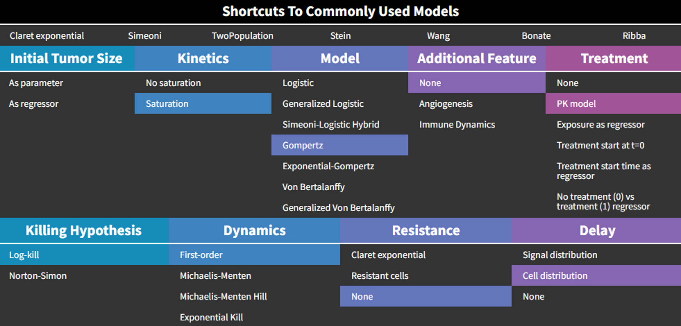
Shortcut models
Lastly, we found that some typical models within the literature. In order to ease access to these models, we created a shortcut tab which automatically leads one to the appropriate selections when applicable, or loads the dedicated model otherwise. In each case, the initial tumor size TS0 can be set as a parameter or as a regressor.
-
Claret exponential model
This model from Claret et al., 2009 corresponds to the following choices in the library:
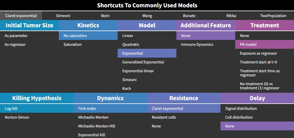
The treatment “PK model” is selected by default, but the Claret model is actually compatible with any type of treatment effect. The version with a constant treatment effect starting at t=0 (choice “Treatment start at t=0”), has an analytical solution implemented in the mode, and is therefore much faster to compute than other models implemented as ODEs
}")
-
Simeoni model
This model from Simeoni et al., 2004 corresponds to the following choices in the library:
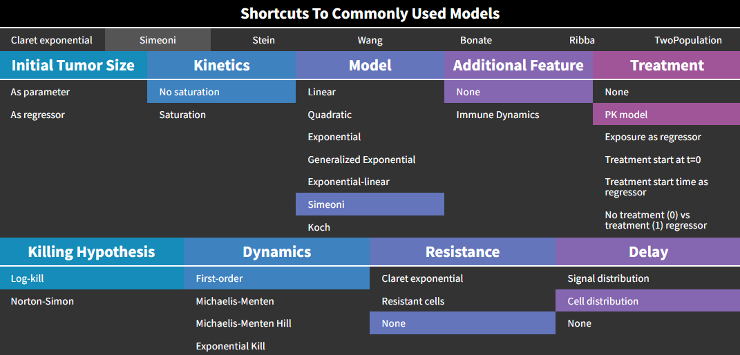
Here again, the treatment “PK model” is selected by default, but the Simeoni model is actually compatible with any type of treatment effect.
The equations are:
=TS0 \\ TS_1(t_0)=0 \\ TS_2(t=0)=0 \\ TS_3(t=0)=0 \\ \frac{dTS}{dt} = \frac{kge*TS}{(1+(\frac{kge}{kgl}*TS)^\psi)^\frac{1}{\psi}} - K*TS \\ \frac{dTS_1}{dt} = \frac{kge*TS}{(1+(\frac{kge}{kgl}*TS)^\psi)^\frac{1}{\psi}} - \frac{TS_1}{\tau} \\ \frac{dTS_2}{dt} = \frac{TS_1 - TS_2}{\tau} \\ \frac{dTS_3}{dt} = \frac{TS_2 - TS_3}{\tau} \\ TotalTS = TS+TS_1+TS_2+TS_3")
-
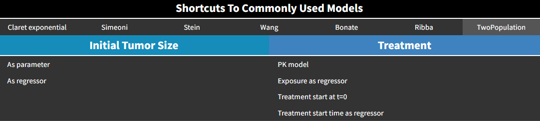
Two-population model
Also called evolutionary model, this simple model corresponds to an exponential growth, and a treatment effect based on log-cell kill hypothesis with first-order kinetics and no delay. The treatment can be set by the user as constant or exposure-dependent.
The equations are:
 \\ TSr_0 = TS0*f \\ \frac{dTS}{dt} = -kkill*EXPOSURE*TS \\ \frac{dTSr}{dt} = kge*TSr \\ TotalTS = TS+TSr")
TS represents the sensitive part of the tumor, and TSr the resistant part. TotalTS is the total tumor size.
If the treatment is constant and starts at time 0, the model is encoded with its analytical solution:
 + (1-f)*exp(-kkill*t))")
with kkill=0 before t=0.
-
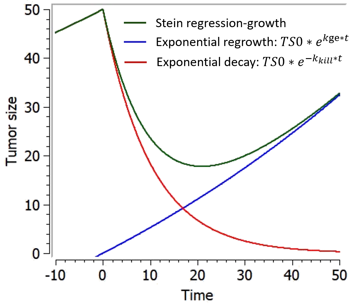
Stein regression-growth model
This model from Stein et al., 2011 is a simple phenomenological equation based on the assumption that the change of tumor size during therapy results from two independent component processes: an exponential decrease/regression and an exponential regrowth of the tumor:
 + exp(kge*t) -1)")
with kkill=0 before t=0.
This model is only available with the treatment option “Treatment start at t=0”.
In responding tumors, regression dominates from start of therapy until nadir, growth dominating after nadir. Theoretical curves depicting the separate components of the model and how these combine together to give the time dependence of the tumor size appear in the figure below.
-
Wang model
This model from Wang et al., 2009 combines an exponential-decay (shrinkage) and a linear-growth (progression). In the original model, the linear growth component is considered as an approximation of tumor growth under a specific treatment, with a treatment-dependent slope. In the present library, the model is implemented with the same linear growth rate before and during treatment. It goes as follows:
+kgl*t")
This model can only be used with the option “Treatment starting at time 0”.
The following figure shows a typical prediction:
-
Bonate model
This model is based on Bonate & Suttle, 2013. It is a modification of the Wang model in which a quadratic growth term has been added to account for curvature of tumor growth following nadir.
It goes as follows:
+kgl*t+kg2*t^2")
-
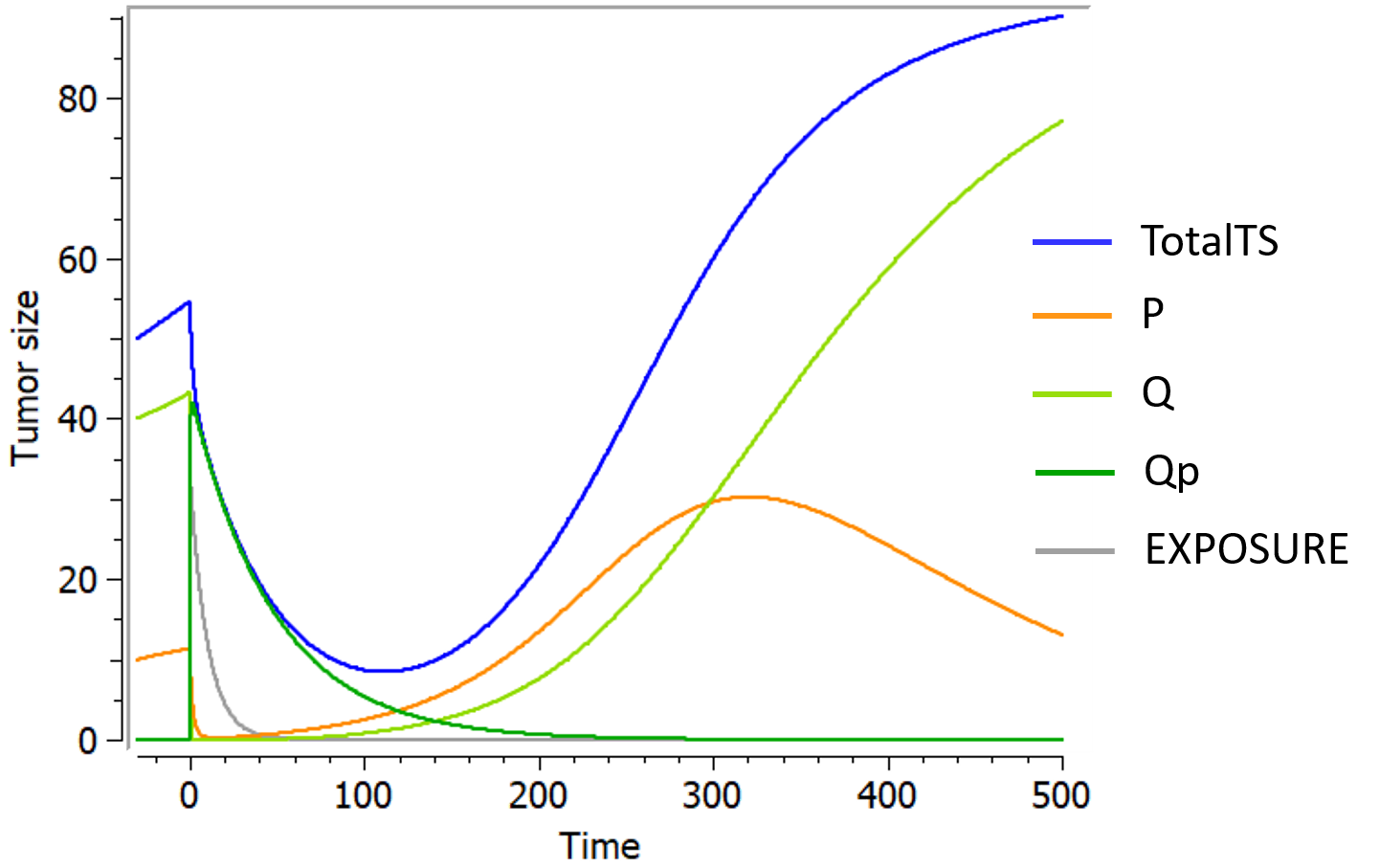
Ribba model
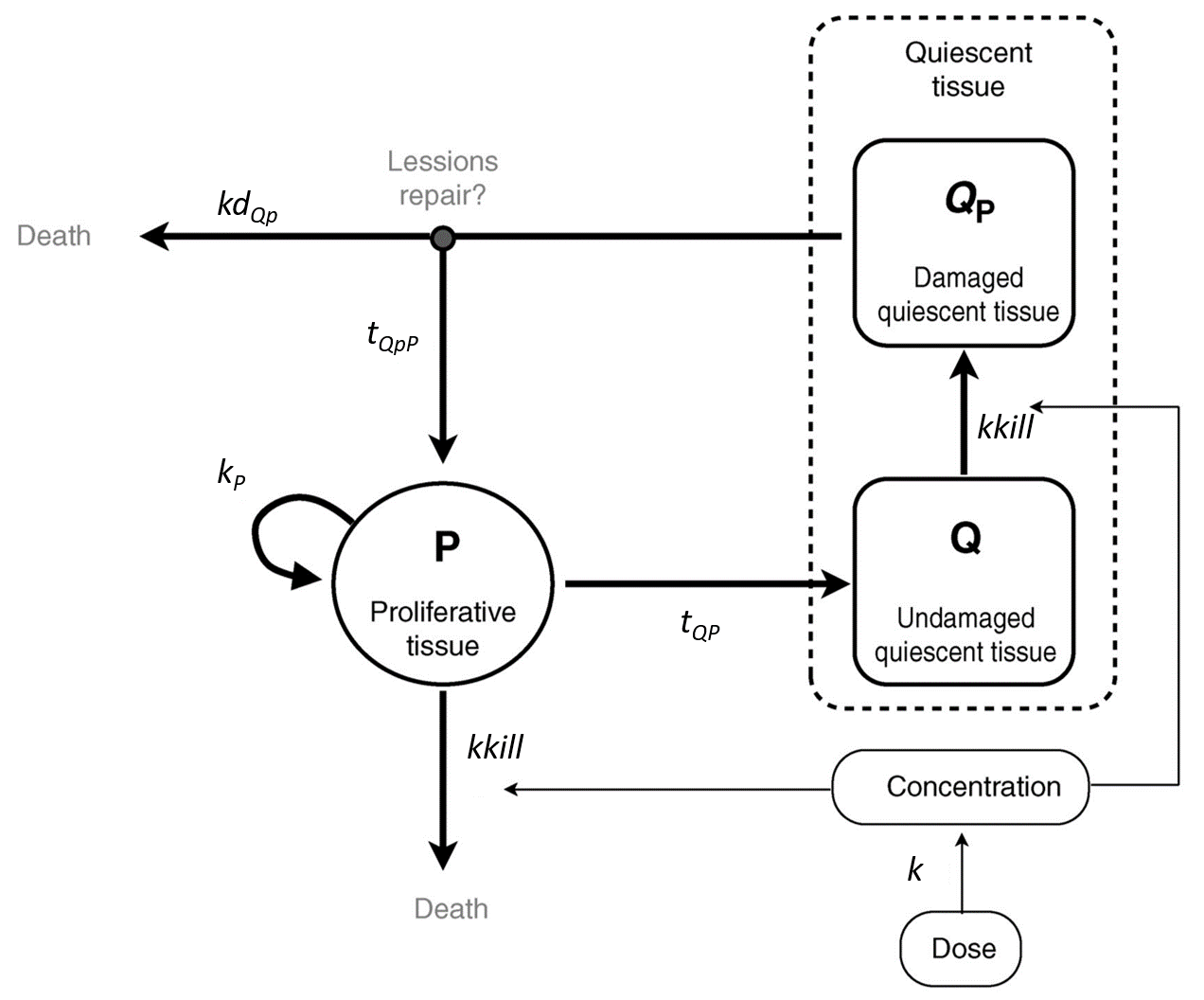
This model has been proposed by Ribba et al., 2012. It is able to capture the growth kinetics of low-grade glioma after termination of chemotherapy, characterized by a frequent decrease in volume despite chemotherapy no longer being administered, by considering delayed action of chemotherapy on quiescent tumor cells. The tumor is represented as proliferative and quiescent tumor tissues that respond differently to treatment. The treatment concentration affects both proliferative and quiescent tissue. The tissue composed of cells in proliferation is directly eliminated because of lethal DNA damages induced by the treatment. Nonproliferative tissue is also subject to DNA damages due to the treatment. When re-entering the cell cycle, the DNA-damaged quiescent cells can either repair their DNA damages and return to a proliferative state or die because of unrepaired damages.
It is represented on this figure adapted from [Ribba et al., 2012]:
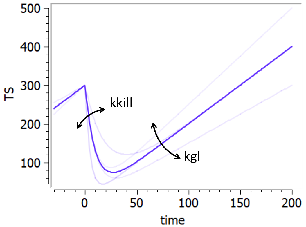
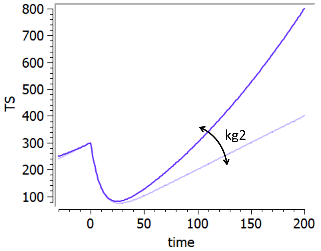
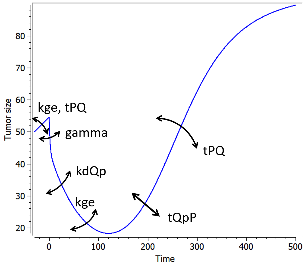
The following curves show the prediction of each variable of the model before and after a treatment dose at time 0, on the left, and the impact of the parameters on the prediction for TotalTS on the right. The treatment concentration causes an initial sharp drop in P and thus in TotalTS, as well as the transfer of cells from Q to Qp. While the treatment concentration decreases then fastly to 0, TotalTS continues decreasing slowly, driven by the elimination of Qp. TotalTS increases again only once enough cells have been transferred from Qp to P. The growth function chosen in this model includes a saturation with a carrying capacity TSmax.
References
Reviews
- Bernard, A., Kimko, H., Mital, D., & Poggesi, I. (2012). Mathematical modeling of tumor growth and tumor growth inhibition in oncology drug development. Expert Opinion on Drug Metabolism and Toxicology, 8(9), 1057–1069.
- Ribba, B., Holford, N. H., Magni, P., Trocóniz, I., Gueorguieva, I., Girard, P., Sarr, C., Elishmereni, M., Kloft, C., & Friberg, L. E. (2014). A Review of Mixed-Effects Models of Tumor Growth and Effects of Anticancer Drug Treatment Used in Population Analysis. CPT Pharmacometrics Syst. Pharmacol.
- Benzekry, S., Lamont, C., Beheshti, A., Tracz, A., Ebos, J. M. L., Hlatky, L., & Hahnfeldt, P. (2014). Classical Mathematical Models for Description and Prediction of Experimental Tumor Growth. PLoS Computational Biology.
- Yin, A., Moes, D. J. A. R., Hasselt, J. G. C., Swen, J. J., & Guchelaar, H. (2019). A Review of Mathematical Models for Tumor Dynamics and Treatment Resistance Evolution of Solid Tumors. CPT: Pharmacometrics & Systems Pharmacology, 720–737.
- Al-Huniti, N., Feng, Y., Yu, J., Lu, Z., Nagase, M., Zhou, D., & Sheng, J. (2020). Tumor Growth Dynamic Modeling in Oncology Drug Development and Regulatory Approval: Past, Present, and Future Opportunities. CPT: Pharmacometrics and Systems Pharmacology, 1–9.
Models from literature
- Simeoni, M., Magni, P., Cammia, C., De Nicolao, G., Croci, V., Pesenti, E., Germani, M., Poggesi, I., & Rocchetti, M. (2004). Predictive pharmacokinetic-pharmacodynamic modeling of tumor growth kinetics in xenograft models after administration of anticancer agents. Cancer Research, 64(3), 1094–1101.
- Koch, G., Walz, A., Lahu, G., & Schropp, J. (2009). Modeling of tumor growth and anticancer effects of combination therapy. Journal of Pharmacokinetics and Pharmacodynamics, 36(2), 179–197.
- Haddish-Berhane, N., Shah, D. K., Ma, D., Leal, M., Gerber, H. P., Sapra, P., Barton, H. A., & Betts, A. M. (2013). On translation of antibody drug conjugates efficacy from mouse experimental tumors to the clinic: A PK/PD approach. Journal of Pharmacokinetics and Pharmacodynamics, 40(5), 557–571.
- Wheldon, T.E., 1988, Mathematical Models in Cancer Research, Adam Hilger, Bristol.
- von Bertalanffy, L. (1957). Quantitative Laws in Metabolism and Growth. The Quarterly Review of Biology, 32(3), 221–233.
- Claret L, Girard P, Hoff PM, Van Cutsem E, Zuideveld KP, Jorga K, Fagerberg J, Bruno R. Model-based prediction of phase III overall survival in colorectal cancer on the basis of phase II tumor dynamics. J Clin Oncol. 2009 Sep 1;27(25):4103-8.
- Hahnfeldt, P., Panigrahy, D., Folkman, J., & Hlatky, L. (1999). Tumor development under angiogenic signaling: A dynamical theory of tumor growth, treatment response, and postvascular dormancy. Cancer Research, 59(19), 4770–4775.
- Hahnfeldt, P., Folkman, J., & Hlatky, L. (2003). Minimizing long-term tumor burden: The logic for metronomic chemotherapeutic dosing and its antiangiogenic basis. Journal of Theoretical Biology, 220(4), 545–554.
- de Pillis, L. G., Gu, W., Fister, K. R., Head, T., Maples, K., Murugan, A., Neal, T., & Yoshida, K. (2007). Chemotherapy for tumors: An analysis of the dynamics and a study of quadratic and linear optimal controls. Mathematical Biosciences, 209(1), 292–315.
- Desmée, S., Mentré, F., Veyrat-Follet, C., & Guedj, J. (2015). Nonlinear Mixed-effect Models for Prostate-specific Antigen Kinetics and Link with Survival in the Context of Metastatic Prostate Cancer: A Comparison by Simulation of Two-stage and Joint Approaches. The AAPS Journal, 17(3), 691–699.
- Lobo, E. D., & Balthasar, J. P. (2002). Pharmacodynamic modeling of chemotherapeutic effects: Application of a transit compartment model to characterize methotrexate effects in vitro. AAPS PharmSci, 4(4), 212–222.
- Jusko, W. J. (1973). A pharmacodynamic model for cell-cycle-specific chemotherapeutic agents. Journal of Pharmacokinetics and Biopharmaceutics, 1(3), 175–200.
- Sun, Y. N., & Jusko, W. J. (1998). Transit compartments versus gamma distribution function to model signal transduction processes in pharmacodynamics. Journal of Pharmaceutical Sciences, 87(6), 732–737.
- Stein, W. D., Gulley, J. L., Schlom, J., Madan, R. A., Dahut, W., Figg, W. D., Ning, Y. M., Arlen, P. M., Price, D., Bates, S. E., & Fojo, T. (2011). Tumor regression and growth rates determined in five intramural NCI prostate cancer trials: The growth rate constant as an indicator of therapeutic efficacy. Clinical Cancer Research, 17(4), 907–917.
- Wang Y, Sung C, Dartois C, Ramchandani R, Booth BP, Rock E, Gobburu J. Elucidation of relationship between tumor size and survival in non-small-cell lung cancer patients can aid early decision making in clinical drug development. Clin Pharmacol Ther. 2009 Aug;86(2):167-74.
- Bonate, P. L., & Suttle, A. B. (2013). Modeling tumor growth kinetics after treatment with pazopanib or placebo in patients with renal cell carcinoma. Cancer Chemotherapy and Pharmacology, 72(1), 231–240.
- Ribba, B., Kaloshi, G., Peyre, M., Ricard, D., Calvez, V., Tod, M., Čajavec-Bernard, B., Idbaih, A., Psimaras, D., Dainese, L., Pallud, J., Cartalat-Carel, S., Delattre, J. Y., Honnorat, J., Grenier, E., & Ducray, F. (2012). A tumor growth inhibition model for low-grade glioma treated with chemotherapy or radiotherapy. Clinical Cancer Research, 18(18), 5071–5080.
Examples of model extensions
The TGI library implemented in Monolix has no ambition of being exhaustive. If a different or more complex TGI model is needed to capture some tumor size data, it can be convenient to start from a model defined in the library, and edit it to derive a user-custom model, a process that is straight-forward with Monolix. In this section we present a few examples of more complex models from the literature and how they can be built based on a model from the library.
Model for combination therapy
[Soon to come]