This page presents the TMDD model library proposed by Lixoft. It includes an introduction to the TMDD concepts, the description of the library’s content, a detailed explanation of the hierarchy of TMDD model approximations, and guidelines to choose an appropriate model.
You can download the library here. All the models are text files. To use it, extract all in a TMDD folder for example.
- Introduction to TMDD concepts
- The TMDD model library
- Overview of the hierarchy of TMDD models and approximations
- Detailed description of TMDD approximations
- Guidelines to choose an appropriate model
- Typical parameters for TMDD
- Examples of molecules
- Extensions to more complex TMDD models
Introduction to TMDD concepts
The concept of TMDD has been proposed as an explanation to the non-linear behavior (violation of the superposition principle and dose-dependent volume of distribution) displayed by some drugs such as bosentan. The concept was first formulated by Gerhard Levy in
Levy describes the TMDD in the following way: “a considerably larger fraction of the dose of these high-affinity compounds is bound to target sites, enough so that this interaction is reflected in the pharmacokinetic characteristics of the drug.”
Target-mediated drug disposition happens when the binding of the drug to the target influences the drugs distribution and elimination. This is in particular often the case for biologics (see section Examples of molecules), such as monoclonal antibodies for instance (for a review, see for instance Dostalek et al. (2013)), because they are designed to be highly specific and strongly bind to their target. In this case, the drug is eliminated both via usual linear clearance mechanisms, that dominate at high concentrations when the target is saturated, and non-linear target-mediated clearance (via binding and internalization of the drug-target complex), that is mainly visible at low concentrations.
The interplay of these mechanisms results in complex concentration-time curves. To describe the observed data, Mager and Jusko ((2001) JPP 28(6)) have introduced a set of equations that includes:
- the linear elimination of the ligand (elimination rate kel)
- the turnover of the receptor (synthesis rate ksyn, degradation rate kdeg, initial receptor concentration R0=ksyn/kdeg)
- the binding of the ligand to the receptor to form the complex (binding rate kon, dissociation rate koff, dissociation constant KD=koff/kon)
- the internalization of the complex (rate kint)
- (optional) the distribution of the ligand to a peripheral compartment (rates k12 and k21)

A key characteristic of TMDD systems is that the pharmacokinetic behavior depends on the dose. Let us focus on the free ligand concentration-time course with several doses of different magnitudes. In the figure below, we look at the concentration (on log-scale) with respect to time. In addition, we use a bolus administration and a single compartment for the ligand (the two compartment case will be studied later on).
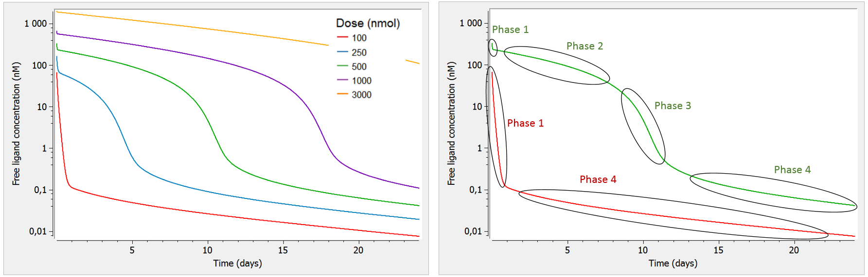
As can be seen on the green curve, when the initial concentration of ligand is larger than the initial receptor concentration (here R0=100), the ligand concentration-time curve displays a complex shape (see also Peletier et al. (2012)) with:
- Phase 1: steep initial decrease, corresponding to the rapid binding of the ligand to the receptor.
- Phase 2: linear elimination phase, where the receptor is saturated with ligands (almost no more binding of ligand to receptor happens), and the ligand is eliminated via usual elimination processes (renal filtration, etc).
- Phase 3: transition phase, where the ligand binds to the no-longer saturated receptor.
- Phase 4: terminal elimination phase, where elimination of the free ligand happens mainly due to internalization (or degradation) of the target/receptor, which shifts the binding equilibrium out of balance leading to new binding of ligand.
Note that we focus on the concentration of the free ligand, such that binding of the ligand to the receptor constitutes an “elimination” mechanism in that it reduces the concentration of free ligand.
On the opposite, as can be seen on the red curve, if the initial ligand concentration is of the same order of magnitude or lower than the receptor concentration (here R0=100), the free ligand concentration time-curve displays two phases:
- Phase 1: steep initial decrease, corresponding to the rapid binding of the ligand to the receptor
- Phase 4: terminal elimination phase, where elimination of the free ligand happens mainly due to internalization (or degradation) of the target/receptor, which shifts the binding equilibrium out of balance leading to new binding of ligand
Note that in this case, the receptor is never saturated with ligand and target-mediated elimination usually dominates over the linear elimination. Thus, the curve goes directly from phase 1 to phase 4.
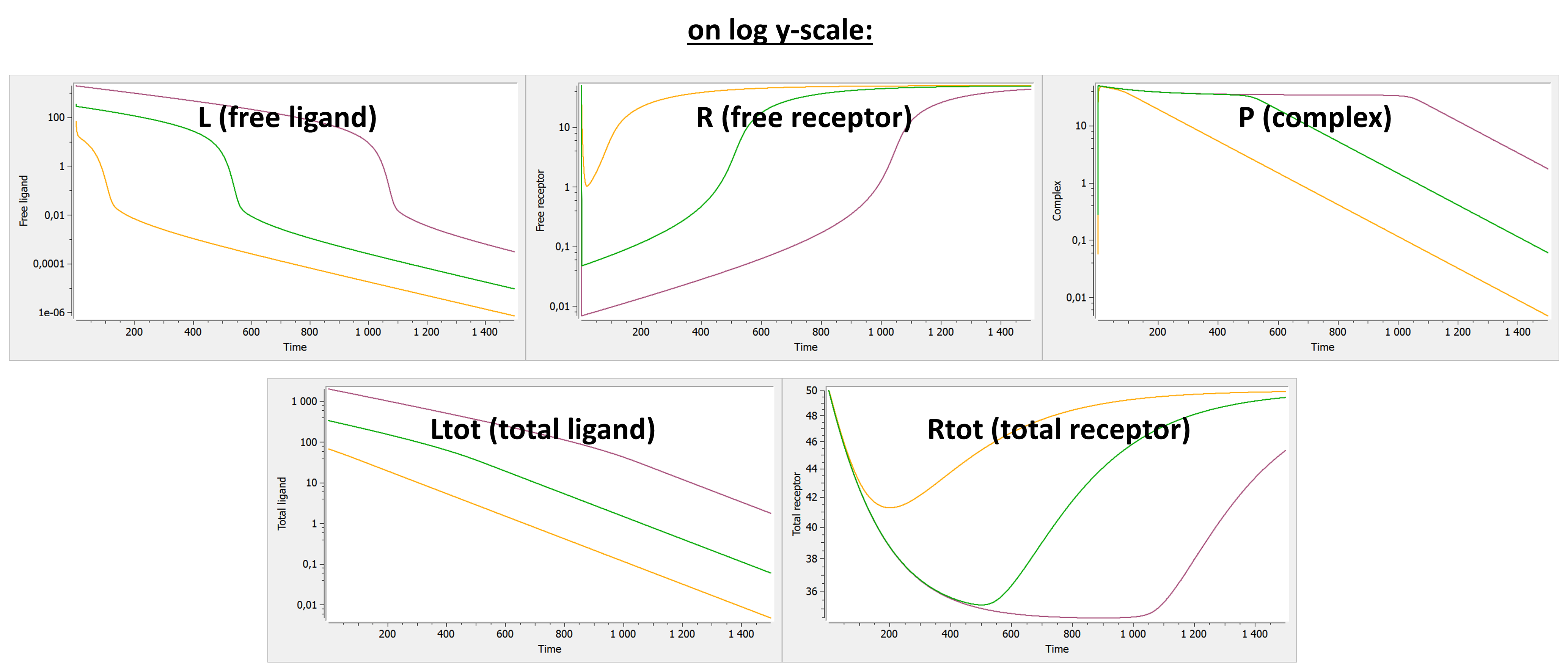
Below we show the typical concentration-time curves for the other entities in linear scale and log scale. The total ligand Ltot is the sum of free ligand L and bound ligand P (complex). The total receptor Rtot is the sum of free receptor R and bound receptor P (complex).

The original TMDD model and its approximations are useful to capture concentration data that display this kind of shapes, or part of them. Below we first describe the content of the library, then we describe the different models and finally give guidelines to choose an appropriate model.
The TMDD library
The library contains a large number of TMDD models corresponding to different approximations, different administration routes, different parameterizations, and different outputs. In total 608 model files are available. The ordering and naming convention permits to easily browse through the list. The file names follow the pattern below:
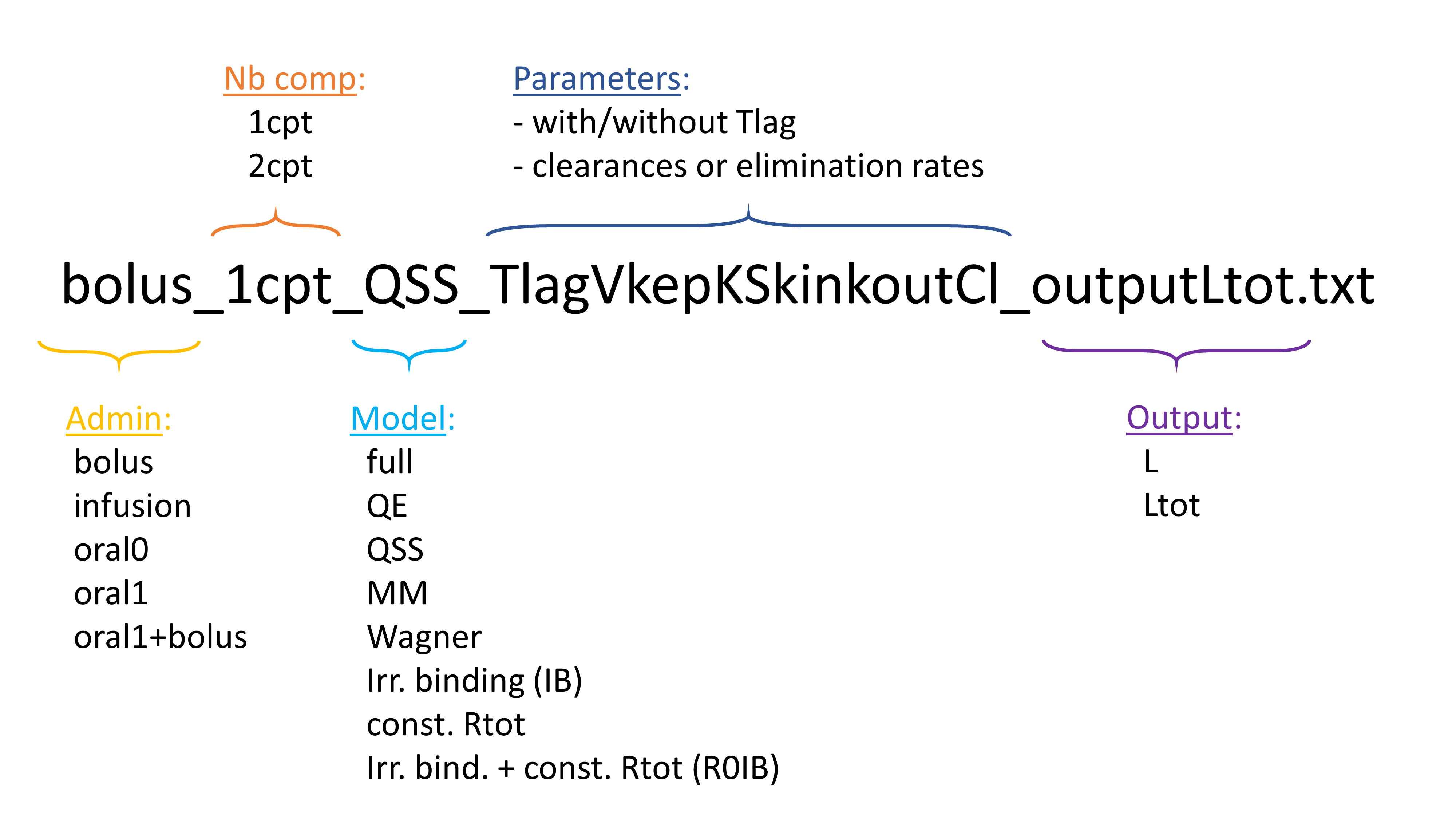
Administration
Five different types of administrations are possible:
- bolus: iv bolus
- infusion: infusion with rate or infusion duration given in the data set (column RATE or TINF)
- oral0: zero-order absorption, with parameter Tk0 for the duration
- oral1: first-order absorption, with parameter ka
- oral1+bolus: first-order absorption or bolus depending on the dose. Bolus doses must be tagged with ADM=1 in the data set and first-order doses (oral or subcutaneous for instance) with ADM=2.
Note that repeated administrations are also allowed. If combinations other than oral1+bolus are necessary, the model file can be duplicated and modified to include a second administration type. In the model, the administration types are distinguished using the type or adm keyword. In the data set, an ADM column must be present.
Number of compartments
All models are available either with 1 compartment or with 2 compartments (central and peripheral). The impact on the model behavior will be detailed in the next section.
Models (approximations)
Beside the original full TMDD system of equations, several approximations have been derived, corresponding to different limit cases. The hierarchy of these approximations and their impact on the model behavior will be detailed in the next section.
Parameters
The list of parameters is mentioned in each file name. The naming convention follows Gibiansky et al. (2008), JPP 35(5). We use the parameters (ksyn, R0) instead of (ksyn, kdeg), and (kon, KD) instead of (kon, koff) because they allow an easier initialization of the parameters. For the elimination and peripheral compartment, two parameterizations are possible, either using clearances or using rates. In addition, a parameter Tlag is available to introduce a time lag for the administration.
Outputs
The model outputs will be matched to the observed data. If only the free ligand L, or the total ligand Ltot have been measured, the files ending with ‘outputL’ and ‘outputLtot’ can be used respectively. If one or several other entities have been measured, the model files must be adapted to output one or several variables in the MARKDOWN_HASHe4fdc9890583978ba7811d0e48b55a31MARKDOWN_HASH section.
If several outputs are present, the outputs will be matched by order with the YTYPEs defined in the data set (first model output matched to observations with YTYPE=1, second model output matched to observations with YTYPE=2, etc). For all models except the Michaelis-Menten TMDD model, the available outputs are the following:
- L: free ligand
- R: free target/receptor
- P: free complex
- Ltot: total (free + bound) ligand
- Rtot: total (free + bound) target/receptor
- TO: receptor occupancy (TO=R/Rtot)
- RR: ratio of free receptor to baseline value (RR=R/R0)
For the Michaelis-Menten TMDD model, only the free ligand L is available as output.
Adapting the models for multiple administration types
Except the oral1+bolus, the models from the library are written for only one administration type per data set. However, they can easily be modified to handle several types of administrations.
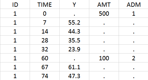
In the data set, the doses must be associated to an administration identifier in the ADM column. In the example below, the first dose is assigned to ADM=1 and the second to ADM=2. Often the CMT column of Nonmem data sets can simply be tagged as ADM column in Monolix.
Using the library model files as a template, the user can then create a new model file adapting the depot statements in the PK: block to its need. In the case of iv and sub-cutaneous administrations, one would write:
PK:
depot(adm=1, target=L, p=1/V) ; doses with ADM=1 in the data set, iv bolus
depot(adm=2, target=L, p=1/V, ka) ; doses with ADM=2 in the data set, first-order absorption with rate ka
For each dose, the depot macro will apply a bolus or first-order input rate to the target L, depending on the ADM identifier of the data set.
Do not forget to include the additional parameters into the MARKDOWN_HASH8d060b1490f65f1cab71b12b99c2985eMARKDOWN_HASH statement.
Download
You can download the library here. All the models are text files. To use it, extract all in a TMDD folder for example.
Overview of the model hierarchy
The figure below gives an overview of the different models, their parameter and the resulting typical concentration-time curve for the free ligand. The assumptions leading from one approximation to another one are also depicted.
The plots represent typical concentration-time curves in log-scale for the free ligand L. The graphics comes from a Mlxplore project defined below. The arrows depict the degrees of flexibility: curved arrows denote that the angle can be changed, while straight arrows denote that the curve can be shifted.
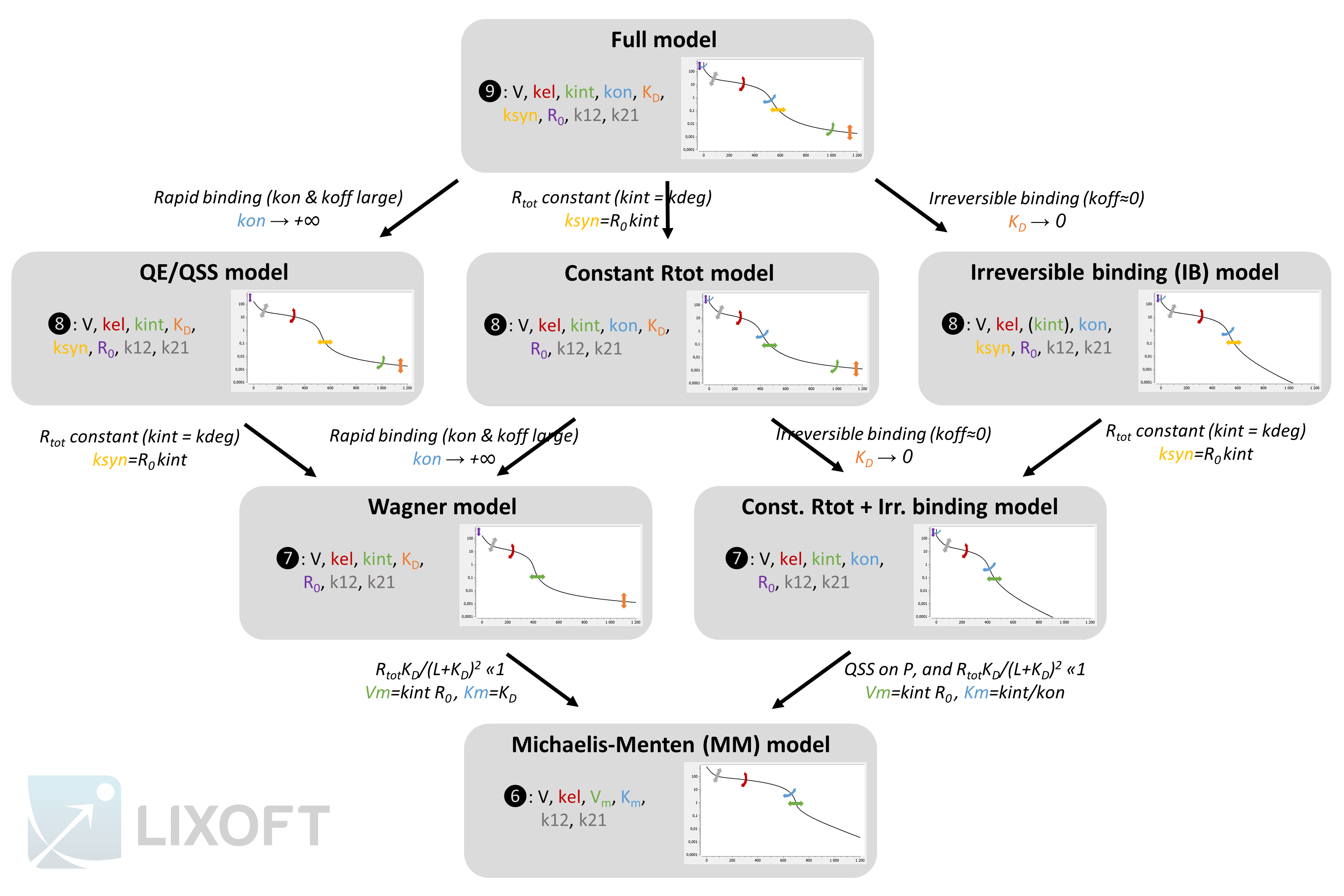
You can use this scheme but you need to cite Lixoft when using it (high quality pdf scheme here). A few comments to better understand the scheme:
- The QE and QSS models are shown together because their system of equations is the same. However the QSS model is derived from the full model using a quasi steady-state assumption. In this case, the name of the new parameter is
.
- The parameters for the second compartment (k12 and k21) influence the non-linear concentration decrease in phase 2, but also the slopes of phase 3 and 4 (which is not depicted for clarity). In the models that lack flexibility in phase 4 (IB, Wagner, MM and const Rtot+IB), some flexibility is present due to k12 and k21 but it is tightly related to the shape of the non-linearity in phase 2.
- In the first and second rows of models, kint influences the slope of phase 4. On the opposite, in the third and fourth rows, kint influences the start time of phase 3, which was previously influenced by ksyn. Note that because
and
, ksyn and kint are related via
.
- The circled numbers represent the number of parameters for a two compartment model. In case of a one compartment model, the number of parameters would be reduced by two. With a single compartment, the phase 2 would be linear. In addition, phase 4 would be completely missing for the IB, MM and const. Rtot+IB models. These curves can be seen in the detailed description section.
- In the IB model, the kint parameter has no influence on the free ligand concentration L, but it has on the total ligand concentration Ltot. If only the free ligand concentration L is measured, the IB and the const. Rtot+IB models are equivalent.
 .
. and
and  , ksyn and kint are related via
  .
.An Mlxplore project allowing to explore simultaneously the behavior of the seven models, for all entities, is available here. Uncomment the lines in the sections <OUTPUT> and <RESULTS> to switch from L to other entities. Uncomment the lines in section <DESIGN> to compare the impact of several dose amounts. Set k12=0 to explore the behavior of a one compartment model. Note that a saturation at 1e-6 was added for some models to avoid infinitely small values in the one compartment case. In the “graphic” tab, in section “Axes”, you can choose between linear or log scale. To change the type of administration, you can adapt the depot macro, add the additional parameter(s) to the input list and give a reference parameter value in the <PARAMETER> section.
Detailed description of the models
For clarity reasons, each model has its own dedicated page. All the links are below.
- Full model
- Rapid binding (QE) and quasi steady-state (QSS) models
- Constant Rtot model
- Irreversible binding model
- Wagner model
- Constant Rtot + irreversible binding model
- Michaelis-Menten (MM) model
Guidelines to choose an appropriate model
The guidelines are given on a separate webpage.
Typical parameters for TMDD
Following the PAGE talk by Leonid Gibiansky, the table below summarizes the typical TMDD parameters, their distribution, their usual range of values, their units, as well as possible covariates: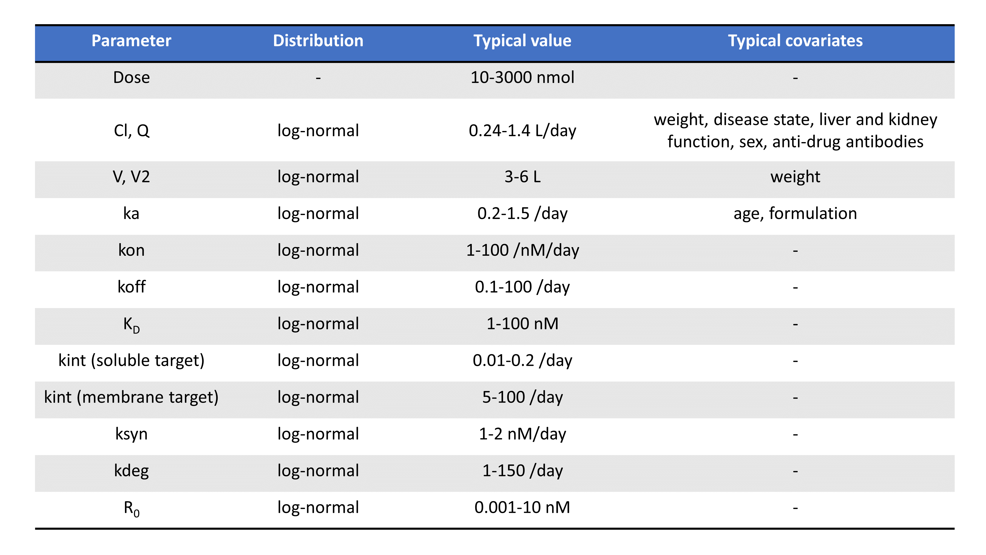
Note that parameters related to the binding (such as Km, KD, kon, koff) depends on the molecule’s chemical properties and are less likely to vary from individual to individual, compared to volumes or parameters that depend on enzyme levels such as kel for instance.
An extensive literature review of parameter values for monoclonal antibodies is also presented in Le Dirks (2010).
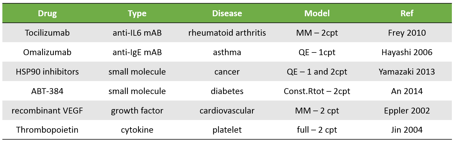
Examples of molecules
The table below presents a few examples of molecules displaying TMDD. Biologics are typical candidates for TMDD but small molecules can also display TMDD kinetics. The models used to describe the kinetics of these molecules range from simple MM TMDD models with one compartment to the full TMDD model with 2 compartments.
Extensions to more complex TMDD models
In this section, we propose links to resources to extend the proposed library of models to more complex TMDD models. The user who wishes to incorporate these extensions can use the library model files as a starting point.
PK/PD modeling
The mechanistic approach used in TMDD models makes it easy to extend the PK model to a PK/PD model and assume that the pharmacological effect is proportional to the concentration of the drug-receptor complex or to the target occupancy. PK/PD models for molecules displaying TMDD kinetics are for instance presented in Bauer et al. (1999), JPB 27(4), or in Mager et al. (2003), JPET 307(3).
Prediction of human PK from animal data
The prediction of the human PK of drugs is a key step for the accurate estimation of doses for first in human clinical trials. Two approaches are often used: allometric scaling and physiologically-based PK models.
Inter-species allometric scaling
To predict human pharmacokinetic parameters values from animal data, inter-species scaling is often used for small molecules. In the most common approach, the PK parameters are related to the body-weight using a power law. This approach is also often used for biologics, although possible species difference in the target must be kept in mind (Glassmann et al. (2016), JPP 43(4)). Successes and limitations are for instance presented in Kagan et al. (2010, Pharm Res 27), and Dong et al. (2011, Clin Pharm 50(2)).
Physiologically-based TMDD models
Physiologically-based pharmacokinetic (PBPK) models extend typical PK models to more compartments that represent the different organs or tissues of the body, with interconnections corresponding to blood flows. The incorporation of the body’s anatomy and physiology in a more detailed way makes it possible to predict human PK by adapting the volumes and flows of the animal body to those of the human body. A quite generic PBPK model for molecules displaying TMDD kinetics is presented in Glassman et al. (2016), JPP 43(3), and applied to four monoclonal antibodies. For three of them, the model could well predict the human PK.
Ligand facilitated target removal
To use ligand facilitated target removal (LFTR) model, presented in Peletier et al. (2021), a small change needs to be made to the full TMDD model available in the TMDD library. ODE line describing ligand behavior needs to be changed to ddt_L = -kel*L – kon*L*R + (koff+kint)*P.
More complex PK TMDD models
The full TMDD model presented here contains a number of implicit assumptions such as no binding in peripheral tissues, only one target, only one ligand, and no presence of endogenous drug amounts. Models have been proposed that alleviate these hypotheses. They are reviewed in Dua et al. (2015), CPT:PSP 4(6) and we here propose a short list of possible extensions:
- binding in the tissue compartment: Lowe et al. (2010), BCPT 106(3).
- multiple targets: Gibiansky et al. (2010), JPP 37(4).
- receptor recycling: Krippendorff et al. (2009), JPP 36.
- immune response: Perez-Ruixo et al. (2013), AAPS journal 15(1).
- drug-drug interactions: Yan et al. (2012), JPP 39(5), and Koch et al. (2017), JPP 44(1).
- endogenous drug present: Koch et al. (2017), JPP.