Enterohepatic circulation (EHC) occurs when drugs circulate from the liver to the bile in the gallbladder, followed by entry into the gut when the bile is released from the gallbladder, and reabsorption from the gut back to the systemic circulation. The presence of EHC results in longer apparent drug half-lives and the appearance of multiple secondary peaks. Various pharmacokinetic models have been used in the literature to describe EHC concentration-time data.
The reference below provides a basic review of the EHC process and modeling strategies implemented to represent EHC.
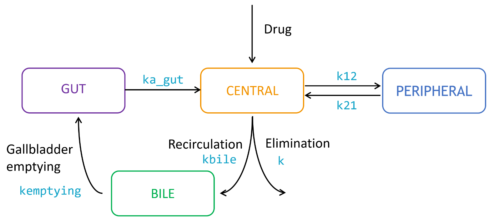
Mlxtran structural model
We present two examples of EHC models, based on a two-compartments model with iv bolus administration. Both models have been implemented with PK macros.
Example with switch function
In the first example, the gallbladder emptying is modelled with a switch function: the emptying rate constant follows a simple piece-wise function, implemented with if/else statements. Hence, gallbladder emptying occurs within time windows, where the rate constant outside these windows is assumed to be zero.
The Mlxtran code for the structural model reads:
[LONGITUDINAL]
input = {V, Cl, Q, V2, kbile, kempt, ka_gut, Tfirst, Tsecond}

PK:
k=Cl/V
k12=Q/V
k21=Q/V2
duration=1
if t>Tfirst & t<Tfirst+duration
kemptying = kempt
elseif t>Tsecond & t<Tsecond+duration
kemptying = kempt
else
kemptying = 0
end

compartment(cmt=1, volume=V, concentration=Cc)
iv(adm=1, cmt=1)
elimination(cmt=1, k)
peripheral(k12, k21)
compartment(cmt=3)
compartment(cmt=4)
transfer(from=1, to=3, kt=kbile)
transfer(from=3, to=4, kt=kemptying)
transfer(from=4, to=1, kt=ka_gut)

OUTPUT:
output = {Cc}
The parameters kbile, kempt and ka_gut describe respectively the transfer rate between the central compartment and the bile, between the bile and the gut, and between the gut and the central compartment.
The parameter kemptying is the rate constant controlling the gallbladder emptying process, and its value changes with time as displayed below:

Here two windows of duration duration=1 have been defined starting at times Tfirst and Tsecond. It is of course possible to extend this model with additional emptying windows, if more than two secondary peaks are noticeable in the data, and to change the value of the parameter duration.
Example with sine function
In the second example, gallbladder emptying is modeled with a sine function, assumed to equal zero outside the gallbladder emptying times. This model accounts for multiple cycles of gallbladder emptying.
The Mlxtran code for the structural model reads:
[LONGITUDINAL]
input = {V, Cl, Q, V2, kbile, kempt, ka_gut, phase, period}

PK:
k=Cl/V
k12=Q/V
k21=Q/V2

kemptying = max(0, kempt * (cos(2*3.14*(t+phase)/period)))

compartment(cmt=1, volume=V, concentration=Cc)
iv(adm=1, cmt=1)
elimination(cmt=1, k)
peripheral(k12, k21)
compartment(cmt=3)
compartment(cmt=4)
transfer(from=1, to=3, kt=kbile)
transfer(from=3, to=1, kt=kemptying)
transfer(from=4, to=1, kt=ka_gut)

OUTPUT:
output = {Cc}
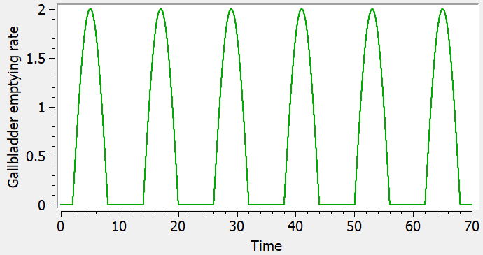
This model assumes fixed intervals between gallbladder release times, with the parameter period defining their frequency. The parameter phase represents the time of the beginning of the first gallbladder release. The value of the parameter kemptying ove time is then:
Variation with oral administration
If the drug administration is oral instead of a bolus, the model can be adapted by replacing the macro iv(adm=1, cmt=1) with absorption(adm=1, cmt=1, ka), which defines a first-order absorption with a rate ka. While ka represents the absorption of the drug, ka_gut represents its reabsorption after storage in the gallbladder. These two physiological processes are not strictly equivalent, as the bile stored in the gallbladder is released into the duodenum. Depending on the drug, ka and ka_gut can be set as separate or identical rate constants.
[LONGITUDINAL]
input = {V, ka, Cl, Q, V2, kbile, kempt, ka_gut, phase, period}

PK:
k=Cl/V
k12=Q/V
k21=Q/V2

kemptying = max(0, kempt * (cos(2*3.14*(t+phase)/period)))

compartment(cmt=1, volume=V, concentration=Cc)
absorption(adm=1, cmt=1, ka)
elimination(cmt=1, k)
peripheral(k12, k21)
compartment(cmt=3)
compartment(cmt=4)
transfer(from=1, to=3, kt=kbile)
transfer(from=3, to=1, kt=kemptying)
transfer(from=4, to=1, kt=ka_gut)

OUTPUT:
output = {Cc}
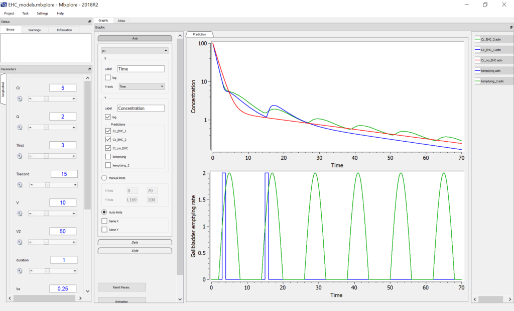
Exploration with Mlxplore
The Mlxplore script below permits to compare the two models with IV bolus, along with the two-compartments model with no EHC.
<MODEL>
[LONGITUDINAL]
input = {V, Cl, Q, V2, kbile, kempt, ka_gut, Tfirst,Tsecond, phase, period}

PK:
k=Cl/V
k12=Q/V
k21=Q/V2

; --- Model with no EHC ---
compartment(cmt=1, volume=V, concentration=Cc_no_EHC)
iv(adm=1, cmt=1)
elimination(cmt=1, k)
peripheral(k12,k21)

; --- EHC model with two constant rate emptying windows ---

if t>Tfirst & t<Tfirst+1
kemptying = kempt
elseif t>Tsecond & t<Tsecond+1
kemptying = kempt
else
kemptying = 0
end

compartment(cmt=3, volume=V, concentration=Cc_EHC_1)
iv(adm=1, cmt=3)
elimination(cmt=3, k)
peripheral(k34=k12, k43=k21)
compartment(cmt=5)
compartment(cmt=6)
transfer(from=3, to=5, kt=kbile)
transfer(from=5, to=6, kt=kemptying)
transfer(from=6, to=3, kt=ka_gut)

; --- EHC model with sine emptying rate ---

kemptying_2 = max(0, kempt * (cos(2*3.14*(t+phase)/period)))

compartment(cmt=7, volume=V, concentration=Cc_EHC_2)
iv(adm=1, cmt=7)
elimination(cmt=7, k)
peripheral(k78=k12, k87=k21)
compartment(cmt=9)
compartment(cmt=10)
transfer(from=7, to=9, kt=kbile)
transfer(from=9, to=10, kt=kemptying_2)
transfer(from=10, to=7, kt=ka_gut)

EQUATION:
odeType=stiff

<PARAMETER>
V=10
Cl=5
Q=2
V2=50
kbile=0.25
kempt=2
ka_gut=0.25
Tfirst = 3
Tsecond=15
phase=7
period=12

<DESIGN>
[ADMINISTRATION]
adm = {type=1, time=0, amount=1000}

<OUTPUT>
list={Cc_no_EHC, Cc_EHC_1, Cc_EHC_2, kemptying, kemptying_2}
grid=0:0.001:70

<RESULTS>
[GRAPHICS]
p1 = {y={Cc_no_EHC, Cc_EHC_1, Cc_EHC_2}, ylabel='Concentration', xlabel='Time'}
p2 = {y={kemptying, kemptying_2}, ylabel='Gallbladder emptying rate', xlabel='Time'}
gridarrange(p1,p2,nb_cols=1)
We obtain the following profiles for the drug concentration in log scale on the top plot below, with no EHC (red), EHC with switch function (blue) and sine function (green). The bottom plot represents the gallbladder emptying rate.