Lifespan based indirect response (LIDR) models have originally been proposed in the field of hematology. The population of cells are described by cell production and cell degradation. The main assumption of LIDR models is that a cell dies when its lifespan expires. This implies that the cell degradation rate is equal to the cell production rate delayed by the lifespan. This assumption differs from classical indirect response model where the cell (or response) degradation is proportional to the cell number (first-order process), independently of the production rate or the lifespan.
LIDR models have been reviewed in detail in:
The implementation of LIDR model makes use of delayed differential equations, which can easily be solved in the MonolixSuite using the delayed differential equation solver. In the following, we will consider a drug with simple exponential decay after a bolus administration and a response R, which can for instance be the number of blood cells.
Mlxtran code for LIDR models
LIDR model for drugs affecting the production rate of the response
In this model, the drug affects the response via an Imax model on the production rate. The equation for the response is:
}{IC50+C(t)} \right) - k_{in} \left( 1 \pm I_{max} \frac{C(t-T_R)}{IC50+C(t-T_R)} \right)")
where + would be used if the drug increases the production rate and – if it decreases it. Notice that the degradation rate is simply the production rate delayed by the lifespan 
")
delay(C,TR) which means that we use the value of the concentration C delayed by time
Note that the delay function makes use of the DDE solver, which is slower than the ODE solver. This video presents an alternative implementation using ODEs only, which leads to greatly shorter run times.
The mlxtran code reads (for the inhibition case):
[LONGITUDINAL]
input={V, k, kin, Imax, IC50, TR}

PK:
depot(target=Ac)

EQUATION:
t_0 = 0
Ac_0 = 0
R_0 = kin * TR

Cc = Ac/V
ddt_Ac = -k*Ac
ddt_R = kin*(1 - Imax *Cc/(Cc+IC50)) - kin*(1 - Imax *delay(Ac,TR)/(delay(Ac,TR)+IC50*V))

OUTPUT:
output = {Cc, R}
As usual, the depot macro permits to link the doses defined in the data set to the DDEs system.
In the model formulation above, it is assumed that both the drug concentration Cc and the response R are recorded in the data set. If only R is observed, the output line should be changed to output= {R}. Note that if the concentration Cc is not observed, it is not possible to identify both V and IC50. The value of V can then be fixed. Alternatively, the K-PD model can be reformulated as in Jacqmin et al. (2007).
In the delay macro, it is mandatory to use an ODE variable. We thus use Ac rather than Cc and divide by the volume V outside of the delay macro.
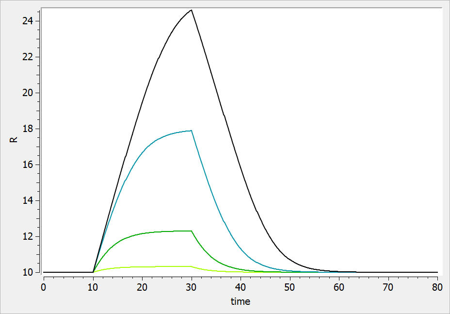
For a drug inhibiting the production rate, the typical response shape is the following (darker colors indicate larger drug amounts). The response start to change from baseline at time 0 and is maximal at time 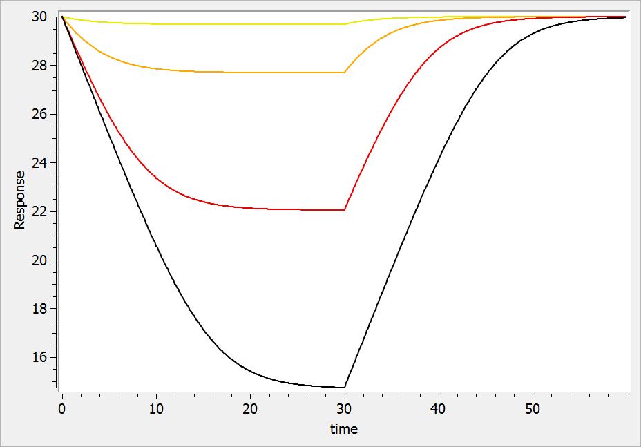
If the drug would increase the production rate instead of decreasing it, the response would increase over time before recovering its basal level: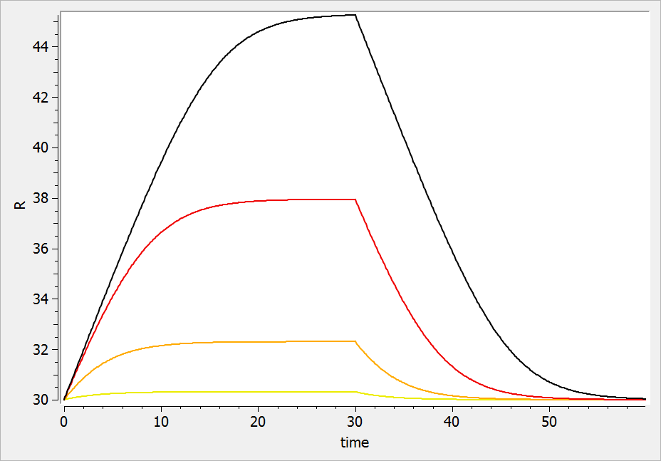
LIDR model for drugs affecting the cell lifespan distribution
This model assumes that initially the lifespan is 
The equation for the response is:
}{IC50+C(t-T_R)} \right) - k_{in} \left( I_{max} \frac{C(t-T_D)}{IC50+C(t-T_D)} \right)")
The mlxtran code reads:
[LONGITUDINAL]
input={V, k, kin, Imax, IC50, TR, TD}

PK:
depot(target=Ac)

EQUATION:
t_0 = 0
Ac_0 = 0
R_0 = kin * TR

Cc = Ac/V
ddt_Ac = -k*Ac
ddt_R = kin - kin*(1 - Imax *delay(Ac,TR)/(delay(Ac,TR)+IC50*V)) - kin*(Imax *delay(Ac,TD)/(delay(Ac,TD)+IC50*V))

OUTPUT:
output = {Cc, R}
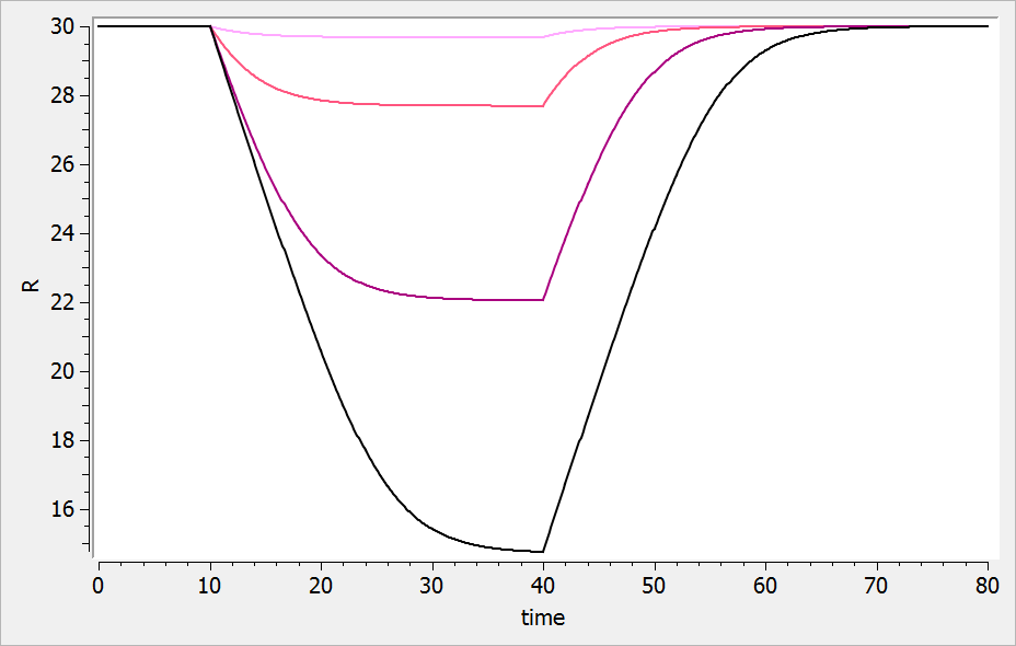
For a drug reducing the lifespan from 

")
")
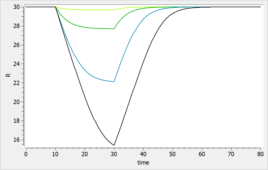
If the drug would increase the lifespan (i.e 
LIDR model with a precursor pool
In this model we assume that the drug effects a precursor pool, which matures into the main pool represented by the response R. Interestingly, it is not necessary to solve the equation for the precursor, only the equation for the response R is needed:
}{IC50+C(t-T_P)} \right) - k_{in} \left( 1 \pm I_{max} \frac{C(t-T_P-T_R)}{IC50+C(t-T_P-T_R)} \right)")
where + is used if the drug increases the precursor production rate and – if it decreases it. 
The mlxtran code reads:
[LONGITUDINAL]
input={V, k, kin, Imax, IC50, TR, TP}

PK:
depot(target=Ac)

EQUATION:
t_0 = 0
Ac_0 = 0
R_0 = kin * TR

Cc = Ac/V
ddt_Ac = -k*Ac
ddt_R = kin*(1 - Imax *delay(Ac,TP)/(delay(Ac,TP)+IC50*V)) - kin*(1 - Imax *delay(Ac,TP+TR)/(delay(Ac,TP+TR)+IC50*V))

OUTPUT:
output= {Cc, R}
The typical response-time curve is displayed below for the case where the drug inhibits the precursor production. The response start to change at time 
If the drug increases the precursor production, we obtain: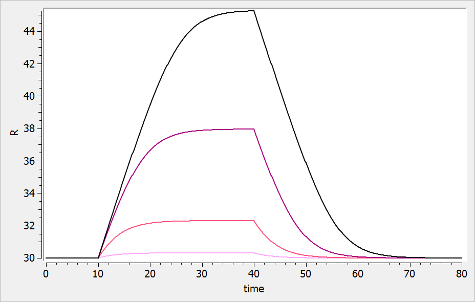
Exploration of indirect model and LIDR model differences with Mlxplore
We explore the differences between:
- the LIDR model
- the indirect response model
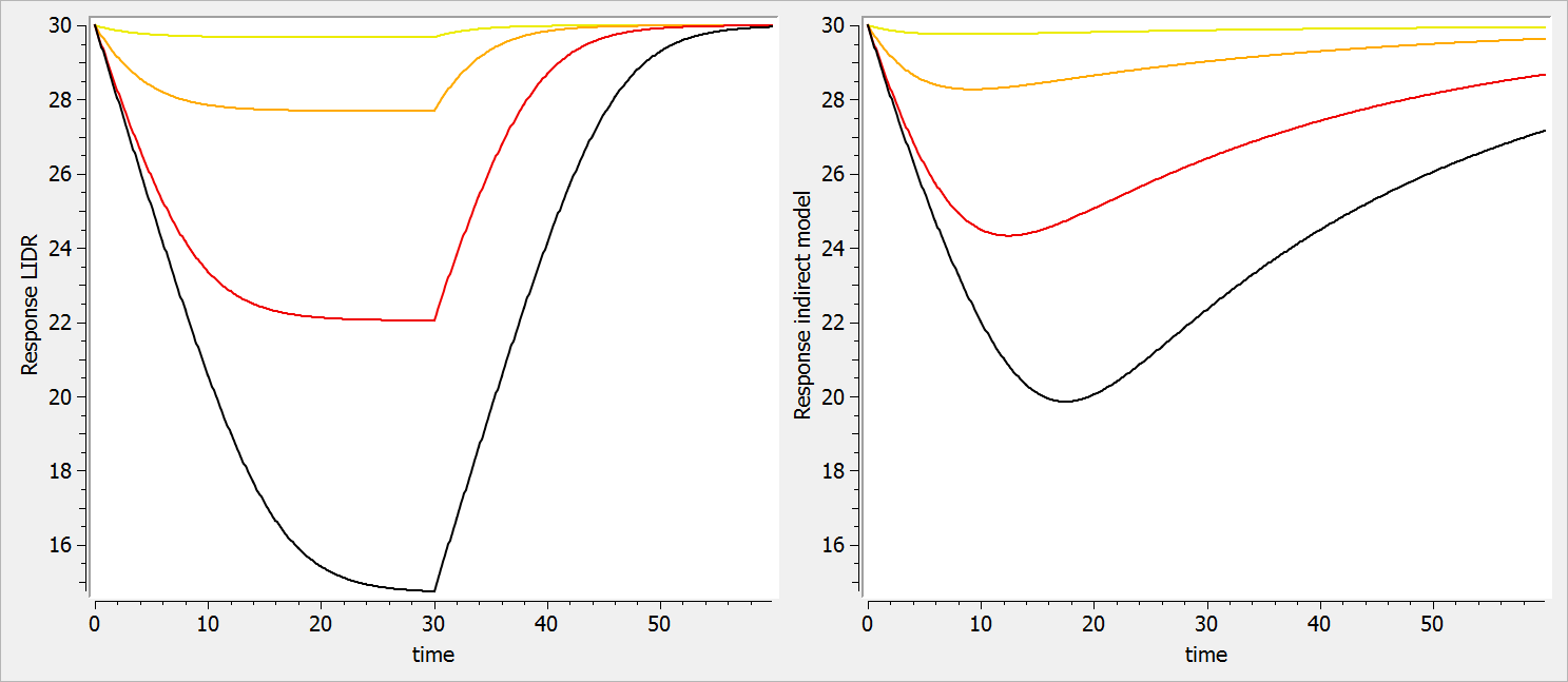
In both models, we assume that the drug inhibits the response production rate. Yet, in the LIDR model, the response degradation rate is equal to the production rate delayed by the lifespan. On the opposite, in the indirect response model, the response degradation rate is proportional to the response magnitude.
In the Mlxplore code below, we have implemented both models with same PK parameters and same production rate kin. To set the same baseline for the two responses, we have assume that the value of the degradation rate for the indirect response model kout is the inverse of the lifespan of the LIDR model.
<MODEL>
[LONGITUDINAL]
input={V, k, kin, Imax, IC50, TR}

PK:
depot(target=Ac)

EQUATION:
; initial values
kout = 1/TR ; to ensure same baseline levels for both
t_0 = 0
Ac_0 = 0
RLIDR_0 = kin * TR
Rind_0 = kin/kout

; drug equations
Cc = Ac/V
ddt_Ac = -k*Ac

; LIDR model
ddt_RLIDR = kin*(1 - Imax *Cc/(Cc+IC50)) - kin*(1 - Imax *delay(Ac,TR)/(delay(Ac,TR)+IC50*V))

; indirect response model
ddt_Rind = kin*(1 - Imax *Cc/(Cc+IC50)) - kout*Rind

<PARAMETER>
V = 10
k = 0.3
kin = 1
Imax = 1
IC50 = 10
TR = 30

<DESIGN>
[ADMINISTRATION]
adm10 = {time=0, amount = 10}
adm100 = {time=0, amount = 100}
adm1000 = {time=0, amount = 1000}
adm10000 = {time=0, amount = 10000}

<OUTPUT>
list={RLIDR,Rind}
grid=0:0.1:60
In the figure below, one can observe how the response for the LIDR model (left plot) plateaus, which is not the case for the indirect model response (right plot). In addition, the peak response time is the same for all drug concentration in the LIDR model but not the in indirect response model. Finally, the relationship between the drug concentration and the extend of the response also differ between the two models.