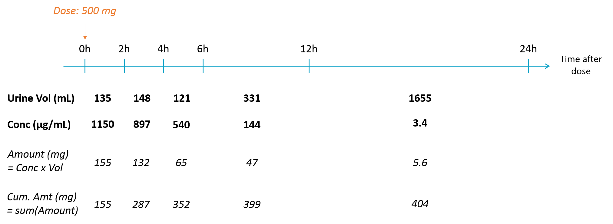
When collecting urine data, the urines are collected over several time intervals. For each time interval, the total urine volume and the drug concentration are recorded. The concentration is not relevant by itself, because it strongly depends on the urine volume that itself depend on how much the individual has drunk etc. We are rather interested in the amount of drug excreted in the urine, which is related to the urinary excretion rate.
The data can be formatted in several ways:
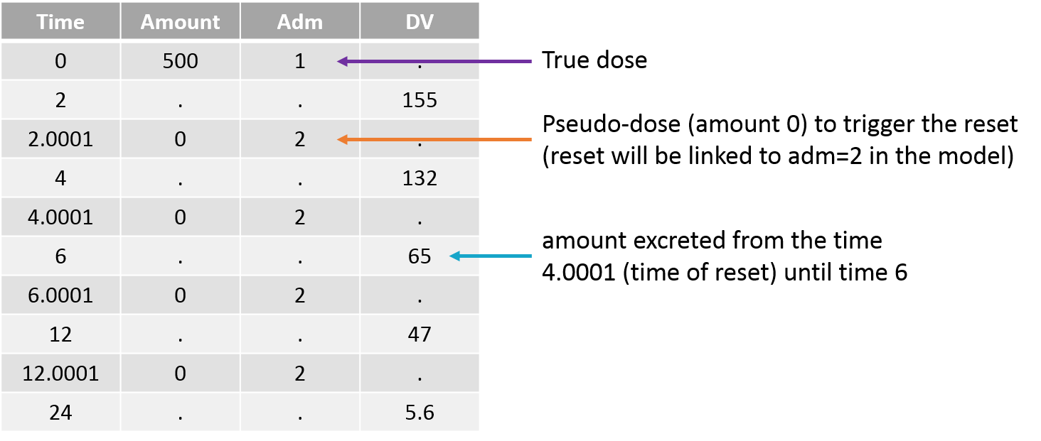
Using the amount
The amount excreted in each interval can easily be computed by multiplying the concentration and the urine volume. When a new interval starts, the “urine compartment” must be emptied, i.e the variable representing the amount excreted in the urine must be reset to zero. To trigger this reset, pseudo-dose records must be added to the data set. They are distinguished from the true doses by a specific administration identifier (here adm=2) and have an amount of 0. To make sure the reset will happen after the observation, the time of the reset are slightly larger than the time of the observation.
For the model, we will assume that the dose arrives in the central compartment and follows a linear elimination with a rate “k”. A fraction “pu” of the drug is eliminated with the kidney and arrives in the urine. The model is written with ODEs in order to be able to apply the resets. True doses (adm=1 in this example) are applied to the variable Aplasma representing the amount in the plasma (central compartment), while pseudo-doses (adm=2) are linked to the empty() macro which resets its target Aurine (amount excreted in the urine) to zero at the time of the pseudo doses. The amount Aurine is outputted to be mapped to the observations of the data set.
[LONGITUDINAL]
input = {k, pu}

PK:
depot(adm=1, target=Aplasma)
empty(adm=2, target=Aurine)

EQUATION:
t_0 = 0
Aplasma_0 = 0
Aurine_0 = 0

ddt_Aplasma = - k * Aplasma
ddt_Aurine = k * pu * Aplasma

OUTPUT:
output = Aurine
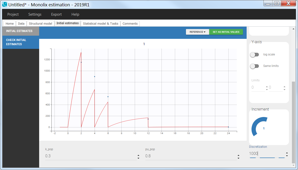
In the “check initial vixed effects” or “individual fits” plot, the resets are clearly visible:

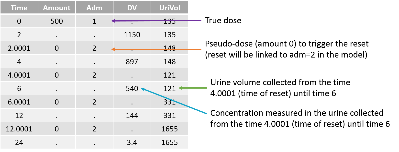
Using the concentration and urine volume
It is also possible to directly use the measured urine volume and drug concentration. The drug concentration is considered as being the observation. To calculate in the predicted drug concentration in the model, the predicted amount excreted in the urine is divided by the urine volume. In order to be passed to the model, the urine volume column in the data set is tagged as regressor. For the parameter estimation in Monolix, only the regressor values on observation lines are important. However, to plot predictions on a regular time grid, Monolix interpolates the regressor values using “Last Observation Carried Forward” and it is necessary to provide a regressor value for the first record (dose or observation line). We thus recommend a provide the urine volume value on all lines.
As when working with the amount, the variable representing the amount excreted in the urine must be reset to zero when a new interval starts. To trigger this reset, pseudo-dose records must be added to the data set. They are distinguished from the true doses by a specific administration identifier (here adm=2) and have an amount of 0. To make sure the reset will happen after the observation, the time of the reset are slightly larger than the time of the observation.
For the model, we will assume that the dose arrives in the central compartment and follows a linear elimination with a rate “k”. A fraction “pu” of the drug is eliminated with the kidney and arrives in the urine. The model is written with ODEs in order to be able to apply the resets. True doses (adm=1 in this example) are applied to the variable Aplasma representing the amount in the plasma (central compartment), while pseudo-doses (adm=2) are linked to the empty() macro which resets its target Aurine (amount excreted in the urine) to zero at the time of the pseudo doses. Before being outputted, the concentration is calculated from the amount in plasma and the urine volume which is indicated as being a regressor and thus read from the data set. Note that the units of the dose, concentration and urine volume must be consistent, or a scaling factor can be added in the model.
[LONGITUDINAL]
input = {k, pu, UriVol}
UriVol = {use=regressor}

PK:
depot(adm=1, target=Aplasma)
empty(adm=2, target=Aurine)

EQUATION:
t_0 = 0
Aplasma_0 = 0
Aurine_0 = 0

ddt_Aplasma = - k * Aplasma
ddt_Aurine = k*pu*Aplasma

Conc = Aurine/UriVol*1000

OUTPUT:
output = Conc
In the “check initial vixed effects” or “individual fits” plot, the resets are clearly visible:
Using the cumulative amount
The cumulative amount can easily be calculated as the sum of the amounts collected from the dose time until the time point of interest. This formatting presents the advantage that no emptying of the urine compartment is necessary. The format of the data set is thus straightforward:
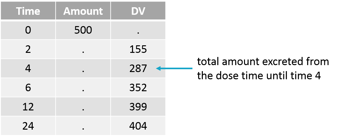
Note that when working with cumulative amounts, if a concentration or urine volume observation is missing, then it is not possible to calculate the cumulative amount for all following time points. Missing information has thus larger consequences than when working with the two other formatting options.
In the model, the cumulative amount is calculated and outputted:
[LONGITUDINAL]
input = {k, pu}

PK:
depot(target = Aplasma)

EQUATION:
t_0 = 0
Aplasma_0 = 0
Aurine_0 = 0

ddt_Aplasma = - k * Aplasma
ddt_Aurine = k*pu*Aplasma

OUTPUT:
output = Aurine
Note that for multiple doses, an emptying of the Aurine variable can be added in the model and in the data set such that the recorded observation represents the cumulative amount from the last dose to the current time.
In the “check initial vixed effects” or “individual fits” plot, the cumulative amount is always increasing (no reset):
