Parent-metabolite models are common and numerous examples exist in the literature. In Bertrand et al. (2011) for instance, parent-metabolite models of increasing complexity are tested for an antipsychotic agent S33138, using Nonmem and Monolix.
Here we present an example of a simple parent-metabolite model. In the model below, the parent compound is absorbed into a central compartment of volume Vp via a first-order process with rate constant ka, diffuse to a peripheral compartment with rates k12 and k21 and is eliminated with a rate kp. The parent compound is also biotransformed into a metabolite with a first-order rate constant kt. The metabolite is eliminated with a rate constant km. The volume of distribution Vm of the metabolite is not identifiable (see below explanation with Mlxplore) and is thus usually fixed to the volume of the central compartment of the parent (Vm=Vp). 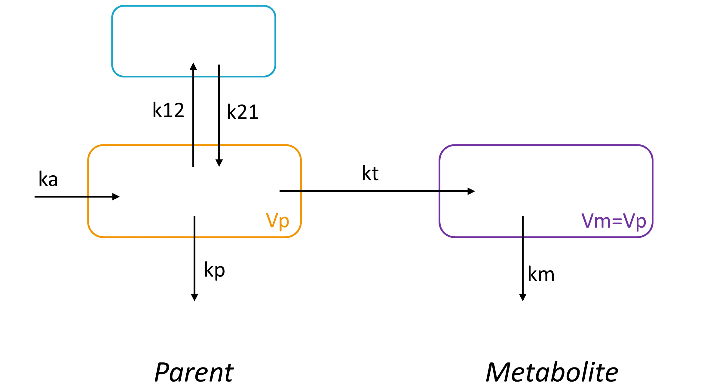
The model can be complexified to take into account a saturation of the biotransformation rate or auto-induction phenomena.
Mlxtran model
The mlxtran code for the structural model reads:
[LONGITUDINAL]
input={ka, Vp, kp, k12, k21, kt, km}

PK:
depot(target=Apc, ka)

EQUATION:
odeType=stiff
t_0 = 0
Apc_0 = 0 ; Apc = amount of parent in central compartment
App_0 = 0 ; App = amount of parent in peripheral compartment
Am_0 = 0  ; Am = amount of metabolite

ddt_Apc = -k12*Apc + k21*App - kp*Apc - kt*Apc
ddt_App = k12*Apc - k21*App
ddt_Am = kt*Apc - km*Am

Cp = Apc/Vp
Cm = Am/Vp

OUTPUT:
output = {Cp, Cm}
The macro depot permits to apply the doses defined in the data set to the ODE system. Here the doses of the data set are applied to the amount of parent in the central compartment via a first-order rate. There is no need to define a depot compartment in the ODE system. All other transfers are defined in the ODE system. The first output of the list (Cp) will be matched to the data with lowest OBSERVATION ID tag (OBSERVATION ID = 1 usually) and the second output (Cm) will be matched to the data with the second OBSERVATION ID tag (OBSERVATION ID = 2 usually). The odeType=stiff line permits to choose an ODE solver designed for stiff systems.
Unidentifiability of Vm explored with Mlxplore
Except when the metabolite has also been administrated, the volume of distribution Vm of the metabolite is not identifiable for the following reason: an increase of Vm can be compensated by a decrease in the biotransformation rate kt, which itself can be compensated by an adjustment of the elimination rate of the parent kp. Note that the disappearance of the parent (via elimination or biotransformation) is driven by ktot=kp+kt and that any combination of kt and kp values that leads to the same ktot will keep the parent concentration-time profile unchanged.
To better grasp this unidentifiability, we propose the following Mlxplore script, where Vm is considered a separate parameter:
<MODEL>
[LONGITUDINAL]
input={ka, Vp, kp, k12, k21, kt, Vm, km}

PK:
depot(target=Apc, ka)

EQUATION:
odeType=stiff
t_0 = 0
Apc_0 = 0
App_0 = 0
Am_0 = 0

ddt_Apc = -k12*Apc + k21*App - kp*Apc - kt*Apc
ddt_App = k12*Apc - k21*App
ddt_Am = kt*Apc - km*Am

Cp = Apc/Vp
Cm = Am/Vm

<PARAMETER>
ka = 1
Vp = 10
kp = 0.1
k12 = 0.05
k21 = 0.05
kt = 0.02
Vm = 15
km = 0.01

<DESIGN>
[ADMINISTRATION]
adm = {time=0, amount=100}

<OUTPUT>
list={Cp, Cm}
grid=0.1:0.1:150
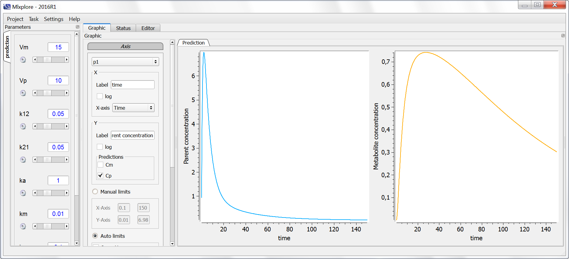
We can then test different values of Vm, kt and kp. The following sets of values (Vm=15, kt=0.02, kp=0.1) and (Vm=30, kt=0.04, kp=0.08) lead to exactly the same prediction for both the parent and the metabolite, highlighting the unidentifiability. One of these 3 parameters must therefore be fixed, the most common choice is to fix Vm to the value of Vp.