Purpose
The elimination macros permits to define different elimination processes (linear or Michaelis-Menten) for compartments. Several eliminations can be defined for the same compartment.
Arguments
Some arguments are common to the two elimination types, while some are specific to a linear or to a Michaelis-Menten type of elimination.
The arguments that are common to linear and Michaelis-Menten are:
- cmt: Label of the compartment emptied by the elimination process. Its default value is 1.
- V: Volume involved in the elimination process. When not specified, its default value is the volume of the compartment defined by cmt.
Additional arguments are needed to define a linear or Michaelis-Menten elimination type.
Arguments specific to a linear elimination
The use of one of the following additional arguments defines a linear elimination:
- k: Rate of the elimination.
- Cl: Clearance of the elimination.
Only one of k or Cl must be defined.
Note, that if no volume has been defined for the compartment and no volume has been defined for the elimination process, then the default volume V=1 is assumed.
Example:
PK:
elimination(cmt=1,k)
Arguments specific to a Michaelis-Menten elimination
The use of both of the following additional arguments defines a Michaelis-Menten elimination:
- Vm: Maximum elimination rate. The unit of Vm is amount/time.
- Km: Michaelis-Menten constant. The unit of Km is a concentration.
Both arguments must be defined.
Example:
PK:
elimination(cmt=1, Vm, Km)
Example with Mlxplore : Comparison of the two eliminations
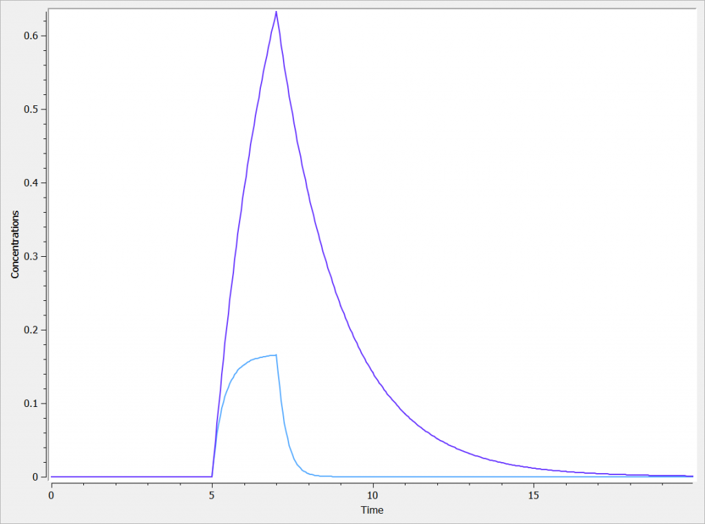
In the following example, the difference between the two elimination processes is demonstrated. The model is implemented in the file elimination.mlxplore.mlxtran, available in the Mlxplore demos and shown below:
<MODEL>
[LONGITUDINAL]
input = {k, Vm, Km}

PK:
compartment(cmt=1, amount=Alin, concentration=Cc_lin)
elimination(cmt=1, k)
iv(cmt=1, adm=1)

compartment(cmt=2, amount=AMM, concentration=Cc_MM)
elimination(cmt=2, Vm, Km)
iv(cmt=2, adm=2)

<DESIGN>
[ADMINISTRATION]
adm_lin = {time=5, amount=1, adm=1, rate=.5}
adm_MM = {time=5, amount=1, adm=2, rate=.5}

<PARAMETER>
k  = .5
Vm  = 2
Km = .5

<OUTPUT>
grid = 0:.05:20
list = {Cc_lin,Cc_MM}

<RESULTS>
[GRAPHICS]
p = {y={Cc_lin,Cc_MM}, ylabel='Concentrations', xlabel='Time'}
The two concentrations are presented in the following figure, with the linear elimination in purple and the Michaelis-Menten elimination in light blue.

One can clearly see the nonlinearities in the Michaelis-Menten elimination process.
Example: PK model with dual elimination pathways
The following model implemented with PK macros includes two compartments, an oral absorption and a dual elimination pathway with parallel linear and Michaelis-Menten eliminations. An equivalent model, implemented with ODEs, is defined in the TMDD model library: it corresponds to the Michaelis-Menten approximation of a TMDD model.
[LONGITUDINAL]
input = {ka, V, Vm, Km, Cl, Q, V2}

PK:
kel = Cl/V
k12 = Q/V
k21 = Q/V2
compartment(cmt=1, concentration=Cc, volume=V)
absorption(cmt=1, ka)
peripheral(k12, k21)
elimination(cmt=1, k=kel)
elimination(cmt=1, Vm, Km)

OUTPUT:
output={Cc}
Rules and Best Practices:
- We encourage the user to use all the fields in the macro to guarantee no confusion between parameters
- Format restriction (non compliance will raise an exception)
- The value after cmt= is necessarily an integer.
- The value after V=, k=, Cl=, Km=, Vm= can be either a double or be replaced by an input parameter. Calculations are not supported.