PK/PD model with effect compartment

Mlxtran structural model

The model can be defined either using the pkmodel macro or a combination of several other macros used as building blocks.

Using the pkmodel macro

[LONGITUDINAL]
input = {ka, V, k, k12, k21, ke0, Emax, EC50, gamma}

PK:
{Cc, Ce} = pkmodel(ka,V,k,k12, k21,ke0)

EQUATION:
Effect = Emax*Ce^gamma/(Ce^gamma+EC50^gamma)

OUTPUT:
output = {Cc, Effect}

The PK part of the model (including the effect compartment) can easily be defined using the pkmodel macro, which infers the model based on the input keywords. With {Cc, Ce} = pkmodel(ka,V,k,k12, k21,ke0), we define a 2-compartment model with first-order absorption and linear elimination, as well as an effect compartment. The concentrations in the central compartment and in the effect compartment are outputted by the macro and can be used to define the PD part of the model.

The PD part of the model (the effect) is defined via an analytical expression which takes into account the concentration in the effect compartment Ce.

Using macros

Instead of using the pkmodel macro, the PK part of the model can also be defined using other macros as building blocks.

[LONGITUDINAL]
input = {ka, V, k, k12, k21, ke0, Emax, EC50, gamma}

PK:
compartment(cmt=1, volume=V, concentration=Cc)
oral(cmt=1, ka)
elimination(cmt=1,k)
peripheral(k12,k21)
effect(cmt=1,ke0,concentration=Ce)

EQUATION:
Effect = Emax*Ce^gamma/(Ce^gamma+EC50^gamma)

OUTPUT:
output = {Cc, Effect}

Model exploration using Mlxplore

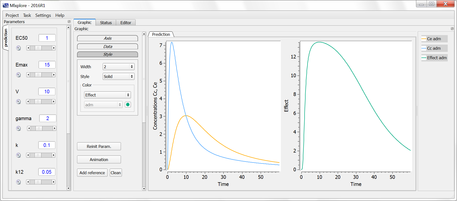
The Mlxplore script including the parameter values, administration design (here one dose) and output reads:

<MODEL>
[LONGITUDINAL]
input = {ka, V, k, k12, k21, ke0, Emax, EC50, gamma}

PK:
{Cc, Ce} = pkmodel(ka,V,k,k12, k21,ke0)

EQUATION:
Effect = Emax*Ce^gamma/(Ce^gamma+EC50^gamma)

OUTPUT:
output = {Cc, Effect}

<PARAMETER>
ka = 1
V = 10
k = 0.1
k12 = 0.05
k21 = 0.05
ke0 = 0.1
Emax = 15
EC50 = 1
gamma = 2

<DESIGN>
[ADMINISTRATION]
adm = {time=0, amount=100}

<OUTPUT>
list={Cc,Ce,Effect}
grid=0:0.1:60

<RESULTS>
[GRAPHICS]
p1 = {y={Cc,Ce}, ylabel='Concentrations Cc, Ce', xlabel='Time'}
p2 = {y={Effect}, ylabel='Effect', xlabel='Time'}

Below we visualize the impact of a reduction of the parameter ke0, leading to a longer delay in the appearance of the compound in the effect compartment:

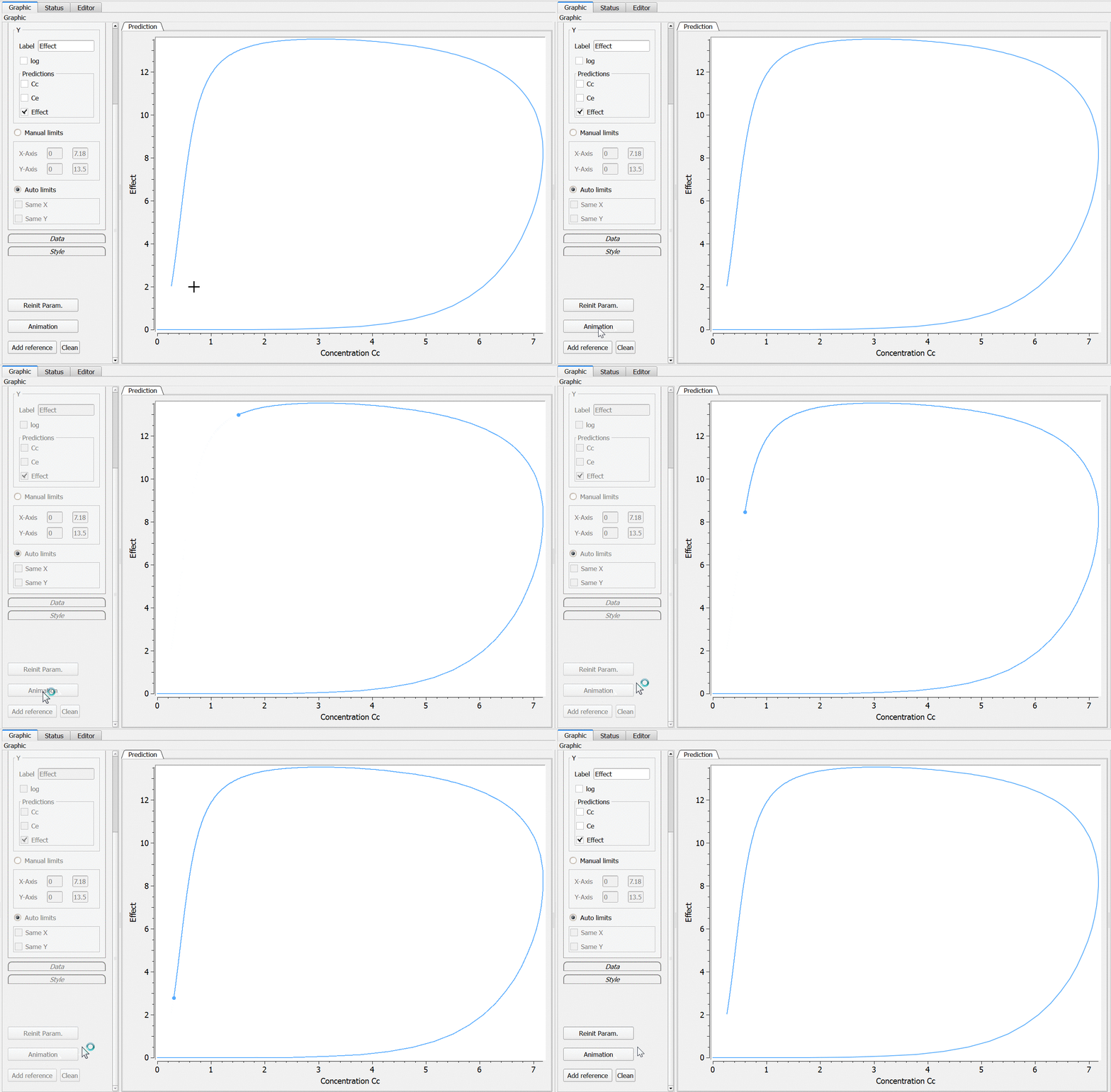
One can also plot the effect with respect to the concentration in the central compartment by changing the <RESULTS> section to:

<RESULTS>
[GRAPHICS]
p1 = {y={Effect}, x={Cc}, ylabel='Effect', xlabel='Concentration Cc'}

Using the ‘animation’ button, the hysteresis characteristic of delayed responses can be visualized: