We here present the system of equation corresponding to the QE and QSS TMDD models, as well as the model behavior.
Rapid binding equations
The steep initial decrease (Phase 1) of the free ligand concentration in the full model usually occurs on a very short time-scale (minutes to hours) compared to the other phases (elimination over days or weeks). If the acquired data starts only after this initial phase, the parameters associated with the binding (especially kon) may not be identifiable. This is why the rapid-binding (also called quasi-equilibrium) approximation has been proposed.
The first derivation has been detailed in Mager & Krzyzanski (2005), Pharm Res 22(10), while a more mathematically rigorous derivation can be found in Koch et al. (2016). JPP. In brief, it is assumed that binding and dissociation of the ligand and target is much more rapid than the other processes, such that the free ligand, free receptor and the complex are at quasi-equilibrium: with
the dissociation constant. To derive a new set of equations, it is convenient to introduce the total ligand concentration
and the total receptor concentration
. Below we present the equations using these quantities, which are the most common ones, but other equivalent formulations are also possible (see Koch et al. (2016). JPP).
As before, V is the volume of the central compartment for the ligand, kel the linear elimination rate for the ligand, KD the dissociation rate, ksyn the synthesis rate for the target/receptor, kdeg its degradation rate, and kint the degradation rate of the complex. In(t) represents the input function, corresponding to the input rate (amount per unit time) of the ligand into the central compartment due to the ligand administration.
In the library model file, a slightly different parameterization is used using the steady-state initial receptor concentration (which replaces kdeg in the list of parameters). This permits to better separate the effect of each parameter.
The complex concentration can be calculated via and the free receptor concentration can be calculated via
.
As for the full model, the system can be extended with a peripheral compartment, leading to:
with A the amount of ligand in peripheral tissues, k12 the rate of transfert from central to peripheral, and k21 the rate in the opposite direction.
Note that the number of parameters has been reduced by one, as kon and koff have been replaced by KD. The behavior of the rapid-binding approximation will be close to the full model behavior if indeed the binding and dissociation reactions are fast compared to the other reactions.
Quasi steady-state equations
The quasi steady-state approximation has been proposed by Gibiansky et al. (2008, JPP 35(5)) for the same reasons as the rapid-binding approximation: lack of identifiability of the full model for typical data sets.
In the QSS approximation, one assumes that the binding rate is balanced by the sum of the dissociation and internalization rates leading to , i.e
. The behavior of the QSS approximation is close to that of the full model if the binding, the dissociation and the elimination of the complex are fast compared to the other processes.
Again, it is more convenient to work with the total ligand concentration and the total receptor concentration, and the equations read:
The complex concentration can be calculated via and the free receptor concentration can be calculated via
.
And with a peripheral compartment, they read:
Notice that this system of equation is exactly the same as for the rapid binding approximation. The only difference is that the QSS approximation uses , while the rapid binding approximation uses
. The interpretation of the meaning of the parameter K differs, but the behavior of the QSS and rapid binding models are exactly the same.
Model properties
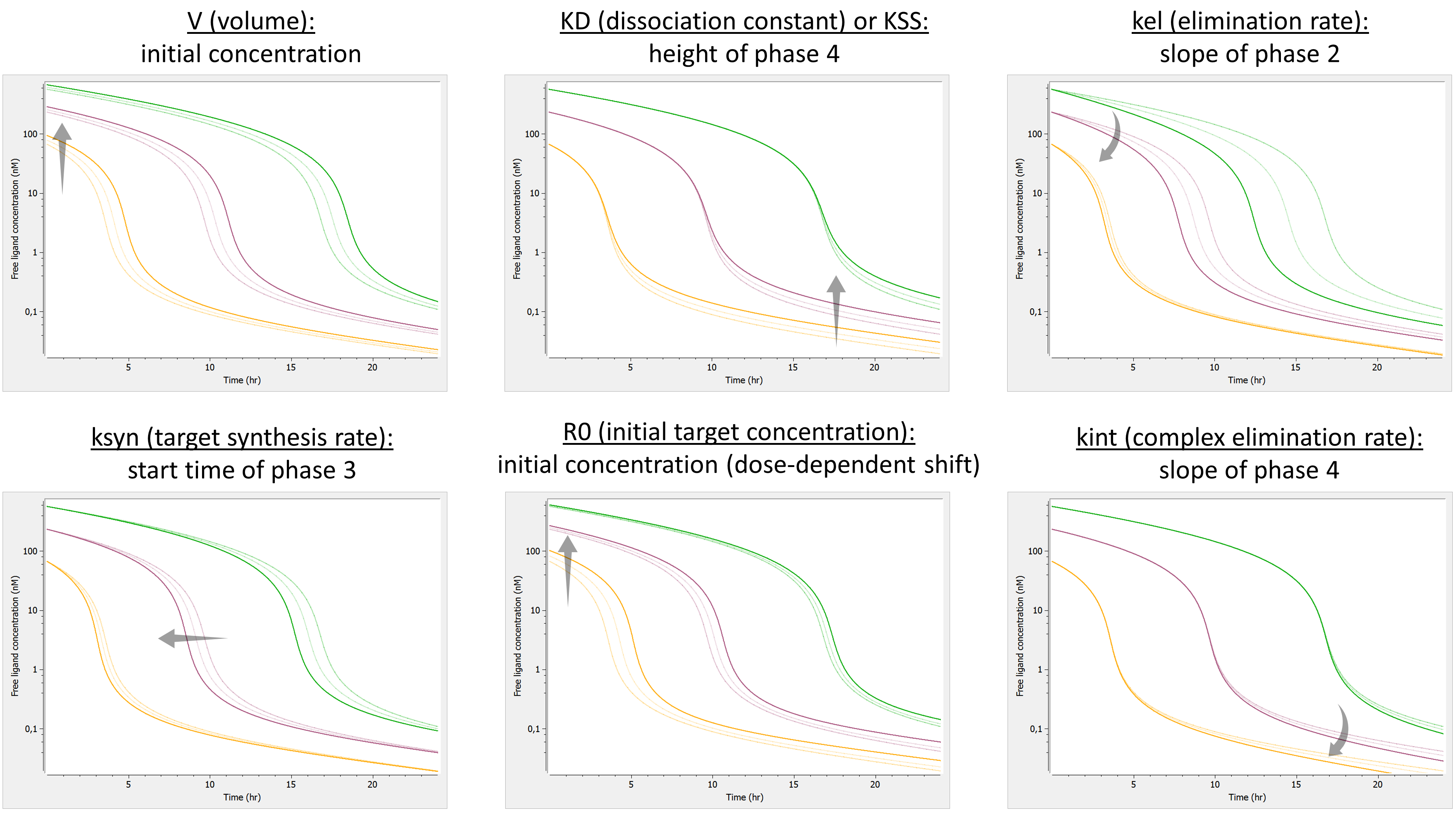
We investigate the influence of each parameter on the typical free ligand concentration-time shape for several dose amounts (bolus administration).

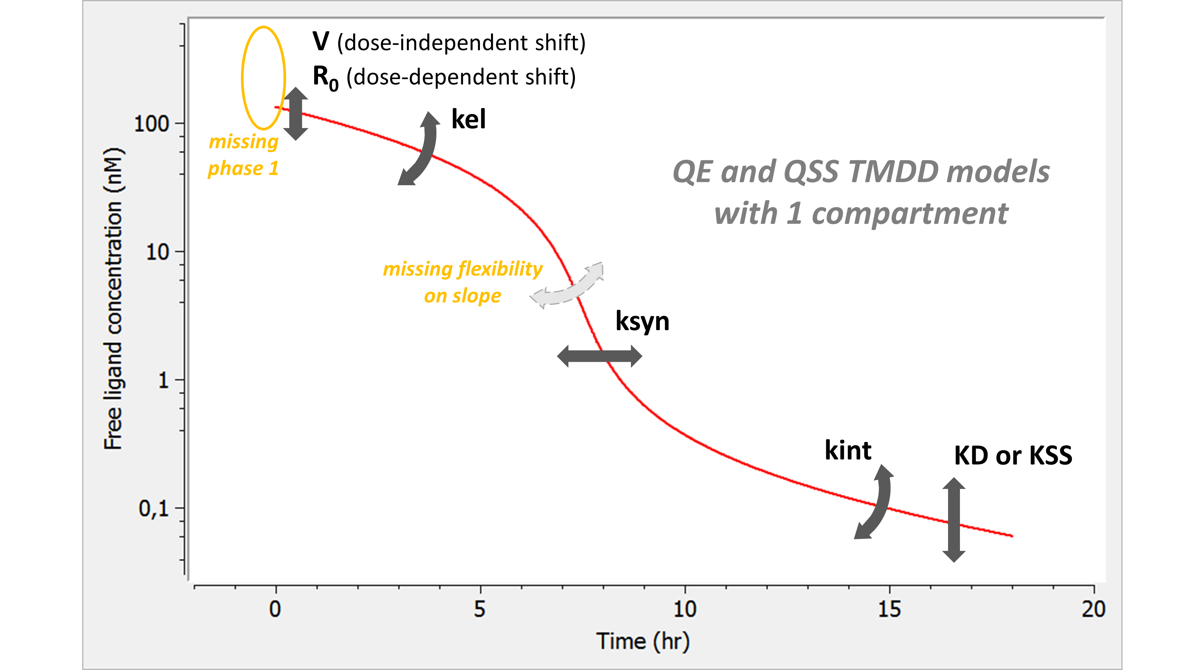
Here is the summary figure:

The phase 1 is completely missing. Indeed, as the binding is assumed infinitely fast, part of the ligand binds immediately to the receptor. In addition, the slope of phase 3 is now fixed with none of the parameters having an influence on it.
Note also that both V and R0 impact the initial concentration. However, whereas a change in V leads to the same shift of the initial concentration for all doses (on a linear scale), a change in R0 shifts the initial concentration of low doses more. If the tested doses do not range over enough orders of magnitude, R0 may be unidentifiable.
Model with 2 compartments
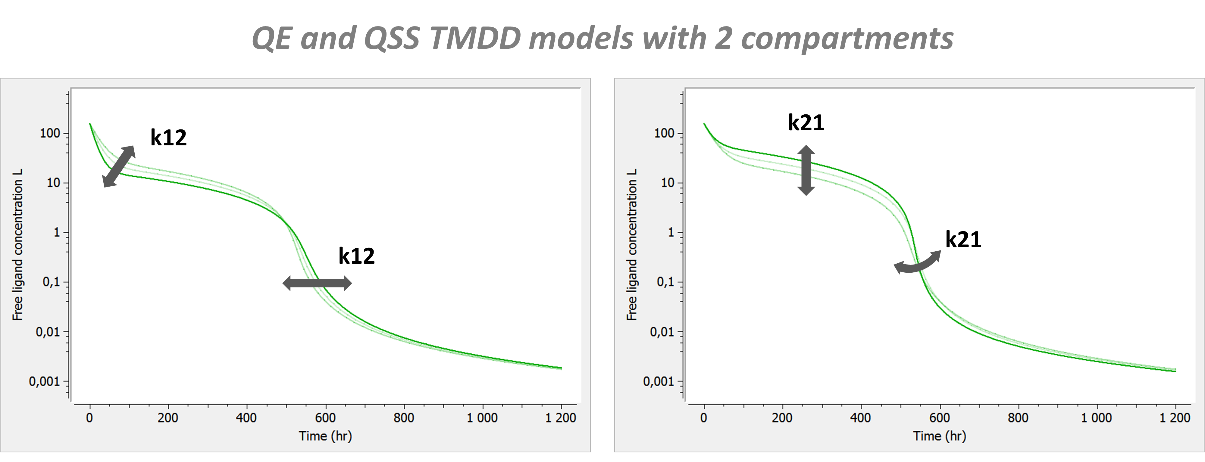
If a second compartment is added, the shape is modified in the following way.

Click here to go back to main TMDD page.